
Optimization Strategy for Electric Vehicle Routing under Traffic Impedance Guidance
by
 ,
,
Jingyu Li
1,2,*, 
Shiyuan Tian
1,*,
Na Zhang
1,2,
Guangchen Liu
1,2,
Zhaoyuan Wu
3 and
Wenyi Li
1,2 1
School of Electric Power, Inner Mongolia University of Technology, Hohhot 010080, China
2
Engineering Research Center of Large Energy Storage Technology, Ministry of Education, Hohhot 010080, China
3
School of Electrical and Electronic Engineering, North China Electric Power University, Beijing 102206, China
*
Authors to whom correspondence should be addressed.
Appl. Sci. 2023, 13(20), 11474; https://doi.org/10.3390/app132011474
Submission received: 23 September 2023
/
Revised: 15 October 2023
/
Accepted: 17 October 2023
/
Published: 19 October 2023
Abstract
:Electric vehicles (EVs) not only serve as significant loads for the power grid but also play a crucial role in the operation of the traffic. Their travel and charging behaviors have an impact on both the power grid and the road network. In order to address the potential impacts of a large-scale deployment of EVs on the power grid and the exacerbation of traffic congestion, this paper first establishes a dynamic road network model based on graph theory and time-varying traffic data combined with a road impedance model. Then, the spatio-temporal distribution characteristics of EV travel are modeled. Furthermore, by incorporating real-time road network data, the traditional Dijkstra’s algorithm for finding the optimal path is improved. At each node, the current real-time road impedance is used as the objective for EV path updates, thus accurately capturing the energy consumption of the EVs. Finally, using a standard testing problem on a typical working day based on data from a real case, the impacts of EV travel and charging behaviors on power distribution network operation and traffic congestion are analyzed under scenarios with no guidance and guidance for the shortest travel time. The results show that this method can significantly reduce the time cost by approximately 18% in travel time, which is of particular concern to users. This method balances the load of the charging stations, elevates the voltage level within the safety requirement of 7%, and simultaneously alleviates traffic congestion near the stations.
1. Introduction
With the development of the economy, the scarcity of fossil fuels, and the worsening environmental pollution, electric vehicles have great potential in the electrification of traffic due to their efficiency, cleanliness, and environmental friendliness [1]. At the same time, with the increasing proportion of renewable energy, there is a higher demand for flexibility in the power system [2]. According to the Notice of the State Council General Office on the issuance of the Development Plan for the New Energy Vehicle Industry (2021–2035), by 2035, the core technologies of new energy vehicles will reach internationally advanced levels, especially in terms of integration with energy, traffic, and information network [3]. With the carbon emissions situation, the electricity market requires the participation of resources such as electric vehicles [4]. Electric vehicles (EVs), as traffic vehicles, first and foremost possess traffic attributes, and due to their flexible charging behavior, the impact of EVs with an increasing penetration rate on the operation of the power grid cannot be ignored.
Due to the different load characteristics in different areas of the city, EVs have different travel characteristics and charging habits. The travel and charging behaviors of EVs simultaneously impact the operation of both the road network and the power grid, realizing the coupling of the traffic network and the power network at charging station nodes. On the one hand, the distribution of the power grid and road network in the area and the level of congestion on road segments determine the travel routes of EVs and the selection of charging stations. On the other hand, the driving and charging behaviors of EVs will simultaneously affect the operation of the power grid and the traffic conditions [5].
In actual operational conditions, the parties involved (EV users, power distribution networks, and traffic networks) often cannot simultaneously maximize benefits or minimize impacts. Due to their individual rationality, EV users make rational route choices based on traffic factors at the time of departure, with their primary goal being to meet their own needs rather than the satisfaction of other participants. Considering the individual rationality of EV users, adopting appropriate strategies to guide EV routes can reduce users’ travel time costs while minimizing the impact on the power grid and alleviating traffic pressure.
In the description of EV characteristics, a modeling method is proposed in [6] to describe the charging method, geographic location, and travel characteristics. In reference [7], the particle swarm algorithm is used to calculate EV energy consumption and analyze the mutual influence between EVs and the power grid. In [8], an EV charging model is established by combining residential travel survey data, considering variations in electricity consumption, and considering travel chains. Ref. [9] develops an EV travel model that incorporates spatio-temporal distribution based on data such as EV daily driving distance, regional land use, and parking distribution. Ref. [10] considered the uncertainty of EV travel and developed an intelligent charging framework for EVs. Ref. [11] considers multiple factors, including the health status of the battery, in order to calculate the residual driving range of EVs. Based on the Markov decision theory, a unit energy consumption model for EVs and a spatio-temporal distribution model for charging behavior are constructed in [12].
In terms of establishing the traffic network models, Ref. [13] utilizes graph theory to describe the topological structure of road networks and introduces an EV speed–flow model. A static road network model composed of distances is constructed in [14], combining real-time operational data of road networks and charging stations to establish a dynamic road network model that considers travel time. In [15], a road network model is established, taking into account segment driving speeds, with charging stations serving as interfaces coupled with the power grid.
Regarding EV travel and charging paths planning, Ref. [16] considers the spatio-temporal characteristics of EVs and the travel time cost of vehicle owners, using Dijkstra’s algorithm to calculate the shortest path between the starting point and the destination or the current location and the charging station. In [17], a multi-agent deep deterministic policy gradient approach is utilized to minimize travel time for the recommendations of charging stations. Combining the Bellman–Ford algorithm, Ref. [18] conducts multi-objective joint charging path planning, minimizing costs and balancing unbalanced traffic flow. In [19], based on graph reinforcement learning, environmental information is extracted to learn fast charging guidance strategies, reduce EV charging time, and balance the operation status of charging stations. Combining real-time data and utilizing the A* algorithm to solve the path for EVs, as described in [20]. In [21], a path optimization scheme is proposed that combines both topographic and traffic information to reduce energy consumption during EV travel.
In the aforementioned studies, certain achievements have been made in the guidance of EV travel. However, there is still potential for improvement in addressing the differences in EV travel demand based on the division of the traffic road network area, analyzing the adverse impacts of EVs on the power grid and transportation, quantitatively describing the factors limiting EV travel during the driving process and combining the shortest path algorithm with the real-time updating of traffic data. Based on the aforementioned research gaps, the main contributions of this paper are as follows:
- Based on graph theory methods and incorporating road impedance models, a dynamic traffic network model with embedded real-time operational data of the road network is established in the context of energy-traffic coupling scenarios.
- After establishing the spatio-temporal characteristics of EV travel, the traditional Dijkstra’s algorithm for optimal path is improved by integrating real-time data from the road network. This enables iterative computation of EV routes, which means that real-time EV path planning is performed at each node considering the current road impedance.
- Taking typical weekday data from a specific region as an example, this study analyzes the demand for EV travel and charging within a 24 h period. It compares the paths without guidance to the paths guided by time (traffic impedance guidance). The aim is to meet user demands and reduce travel costs. The study also analyzes the impact of different EV penetration rates on power distribution voltage levels and traffic congestion in order to validate the effectiveness of the proposed strategy presented in this paper.
2. Establishment of the Electric–Power–Traffic Network Model
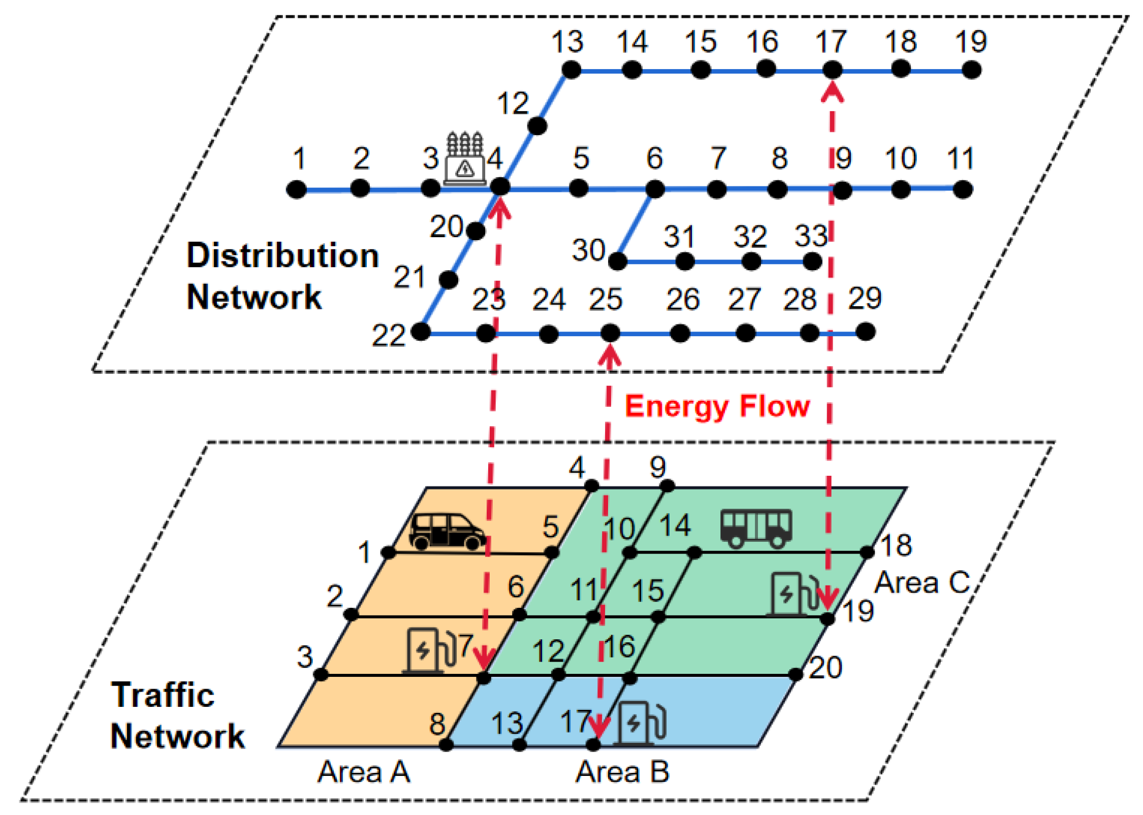
The urban traffic road network serves as the foundation for EV travel, with the road network’s structure and operational conditions impacting various aspects of EV journeys, such as destinations, travel routes, and travel times. Additionally, due to the dual load characteristics of electric power and traffic associated with EVs, the road network’s structure and operational conditions also influence EV charging behaviors, including charge states and charging choices. Consequently, these factors have a certain impact on the operation of the power grid. In other words, the charging behavior of EVs at charging stations establishes power–traffic coupling network between the distribution grid, EVs, and the transportation network, as illustrated in Figure 1.
On the basis of establishing a power–traffic coupling network, it is possible to facilitate information exchange between EVs, the power grid, and the road network. By considering the travel characteristics and charging habits of EV users in different areas of the road network, travel and charging paths can be planned to minimize user travel time costs while meeting their charging needs. This approach aims to reduce the impact of EVs on the power grid and alleviate traffic congestion near charging stations.
2.1. Traffic Network Topological Structure
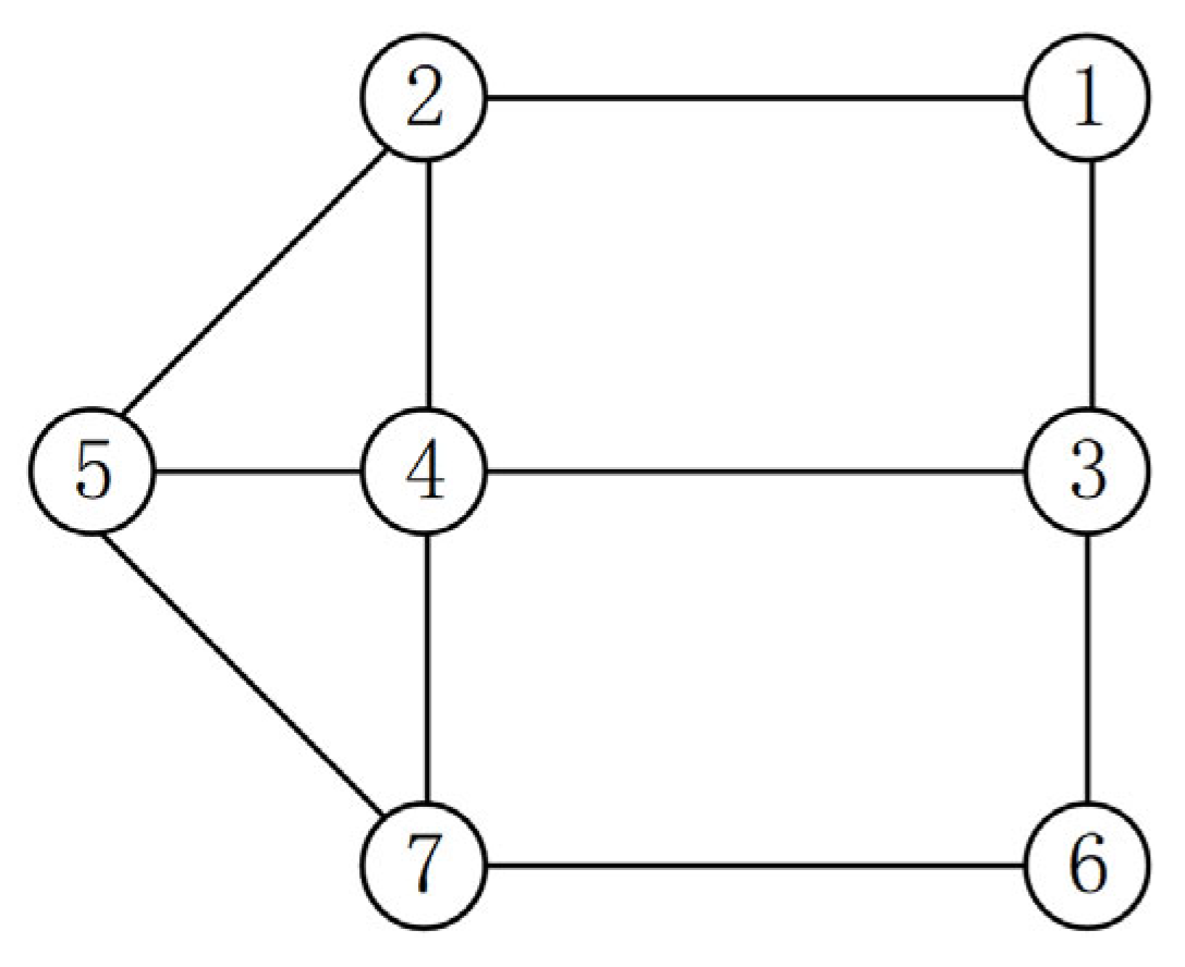
Establishing an appropriate traffic road network model is the foundation for studying EV travel behavior and path selection. The basic road network topology consists of the connectivity between nodes and different roads, as shown in Figure 2.
The basic road network model consists of two elements: nodes and connecting lines. Nodes represent the road intersections in the actual road network, while line segments between nodes represent the various roads connecting the network. The connectivity of the road network is described by the adjacency matrix D, as shown in Equations (1) and (2):
In the matrix D, If node i is connected to node j, the elements at positions (i, j) and (j, i) in the matrix correspond to the length of that road segment. Otherwise, they are represented as ∞.
2.2. Dynamic Traffic Network Model
In the road network topology model described in Section 2.1, the factors influencing vehicle travel are only the node positions and road segment lengths, which constitute a static road network model. However, EVs are often affected by various factors, such as road traffic volume and travel time throughout the day, and the restrictions they encounter during congested and uncongested periods are different. In a static road network, the road lengths do not change with the operating conditions, and considering only the distance of road segments in EV travel paths without considering the real-time traffic conditions can increase user costs and exacerbate traffic congestion. In this paper, we combine real-time traffic operation information of the road network and use graph theory methods to establish a dynamic traffic network model [22], as shown in Equation (3):
In the equation, GT represents the dynamic traffic network, which consists of the following basic elements: V, E, and WT. V represents the set of all nodes in the road network, i.e., road intersections. E represents the set of all road segments in the road network. WT represents the set of weights for each road segment, which quantifies the attributes of the road or the factors restricting vehicle travel. The dynamic road network weights can be quantitatively studied using variables such as varying traffic speeds, travel times, and toll fees. T represents the k time intervals partitioned within a day, with each interval corresponding to different road network operating conditions.
In comparison to the static road network model, the dynamic road network model takes into account the actual operating conditions of the roads at all times of the day. For example, it can use traffic volume at different times of the day and real-time road travel time as road network weights, which can better reflect the factors limiting vehicle travel in actuality compared to just considering the length of the road segments. This allows for a more reasonable guidance of user travel behavior.
2.2.1. Speed–Flow Model
For road travel speed, existing research mostly simplifies its impact by setting it as a constant value. However, in reality, vehicle travel speed is limited by both the road traffic volume and the maximum capacity of the road. This paper considers the influence of real-time traffic volume and establishes a speed–flow model to analyze the real-time travel speed of the road [23], as shown in Equation (4):
The equation consists of the following variables: vij represents the driving speed of an EV on road segment (i,j) at time t; vij0 represents the zero-flow speed of segment (i,j), which is the speed limit for vehicles under free-flow conditions, set as 60 km/h in this paper; Mij denotes the maximum capacity of road (i,j), which varies depending on different road grades; qij represents the real-time traffic flow between nodes i and j at time t; a, b, and c are specific parameters of the model, with values set as a = 1.726, b = 3.15, and c = 3 in this paper. Compared to previous research that assumes a constant driving speed for EVs or determines the driving speed based on a normal distribution, this model calculates the EV driving speed based on the real-time traffic flow on each road segment. As the power consumption of EVs is closely related to driving speed, this model allows for a more accurate estimation of power consumption that varies with road conditions, providing a more precise characterization of energy consumption in EV trips.
2.2.2. Traffic Impedance Model
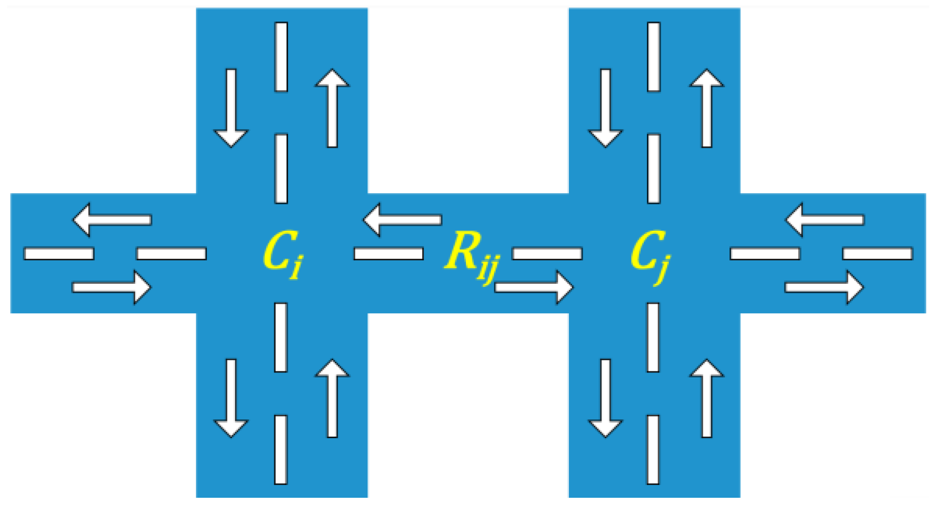
In the quantitative analysis of road weights, traffic impedance is commonly used by transportation agencies to describe the cost of vehicle travel on a road segment, such as travel distance, speed, and time. In static road networks, road segment length is often used as the measure of traffic impedance. However, this approach cannot accurately capture the actual driving conditions of vehicles and cannot provide effective route guidance. In the dynamic road network model presented in this paper, the travel time cost has the most significant impact on user travel behavior. Therefore, a model is introduced where travel time is used as the measure of road impedance. Road impedance includes both road impedance and node impedance [24], as shown in Figure 3.
The road impedance model can be represented as follows:
where wij represents the road impedance, which is composed of node impedance Ci and segment impedance Rij. Rij and Cij are determined by the road traffic saturation level S, which is defined as the ratio of real-time traffic flow qij to the maximum capacity Mij of the road, as shown below:
According to the classification criteria for urban traffic conditions, road conditions can be divided into four levels based on the saturation level S: smooth flowing (0–S–0.6), slow moving (0.6–S–0.8), congested (0.8–S–1), and heavily congested (1–S–2). The impedance models for segment impedance and node impedance corresponding to different saturation levels are as follows:
- Segment Impedance Model
The segment impedance Rij for different saturation levels is represented as follows:
where t0 represents the zero-flow travel time on the road, m and n are the influencing factors of the segment impedance model. The segment impedance model shown in Equation (7) represents the delay in travel time for vehicles in a certain road segment based on the different saturation levels of the segment.
- Node Impedance Model
The node impedance Ci for different saturation levels is represented as follows:
In the equation, g represents the signal cycle, λ represents the green ratio, and q represents the arrival rate of vehicles on the road segment. When vehicles pass through road intersections, they are restricted by traffic signals, resulting in travel time delay, which is known as node impedance, as shown in the above equation.
- Integrated Traffic Impedance Model
Based on the real-time saturation level of the road, the segment impedance and node impedance corresponding to the respective conditions are combined to obtain the time-varying integrated traffic impedance model as shown in Equation (9):
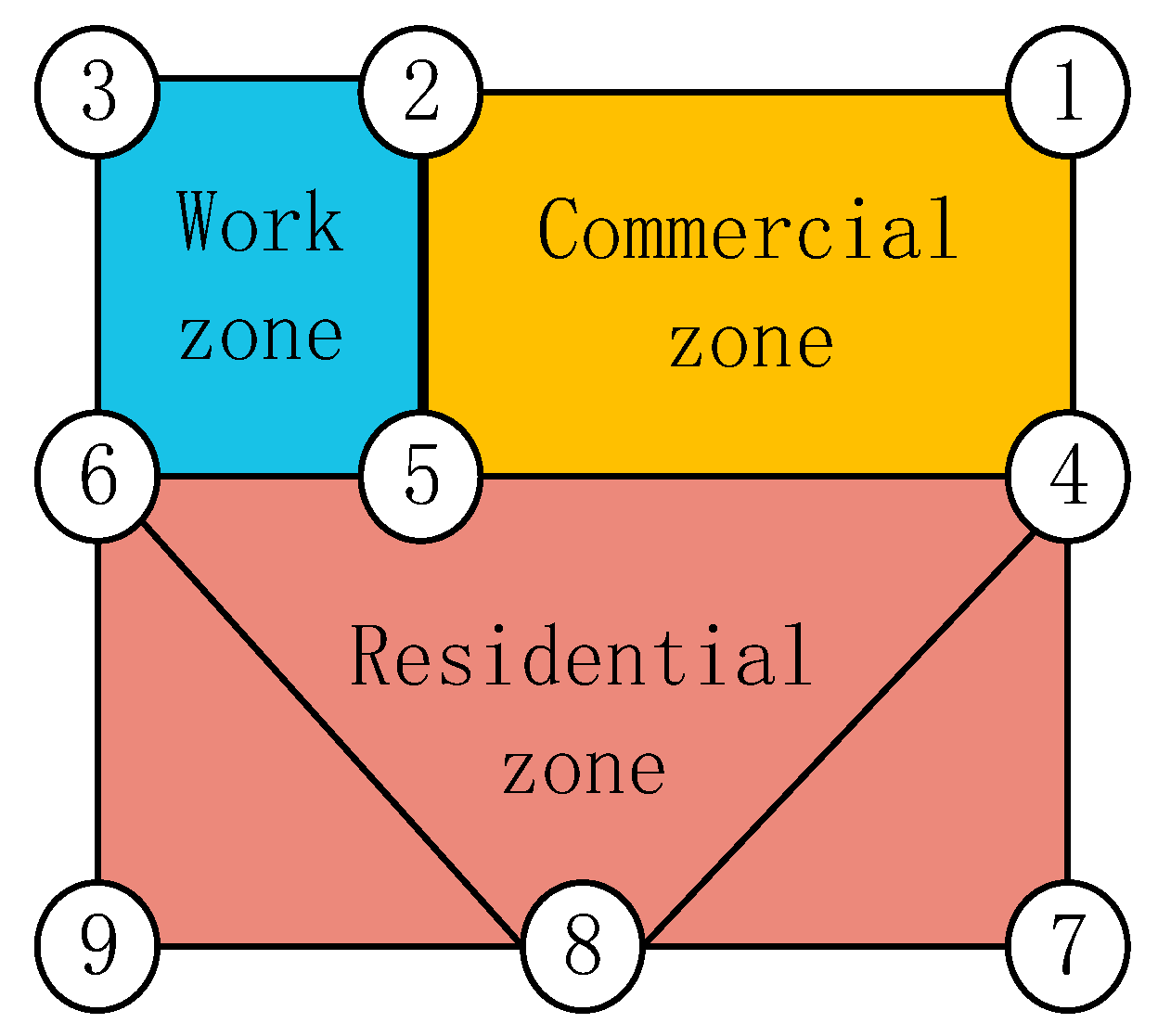
2.3. Network Area Division
The urban area can be divided into residential areas, work areas, and commercial areas based on factors such as load characteristics and user travel characteristics, as shown in Figure 4. Each area includes several transportation nodes and connecting road segments. Residential areas primarily serve as destinations for users with daily life travel needs. Work areas primarily serve as destinations for users with work-related travel needs. Commercial areas primarily serve as destinations for a small portion of users with entertainment travel needs.
2.4. Distribution Network Model
EV achieves the information and energy exchange between the road network and the power grid through charging behavior. Based on the aforementioned dynamic road network model, a distribution network model is established to match it. This paper adopts a standardized distribution network modeling method to establish a 33-node model of a 10 kV distribution network, as shown in Equation (10).
where NP represents node type, voltage, power, etc.; ZP represents node connection relationship, impedance, etc.; and LP represents node location, capacity, etc.
After the EV is connected to the charging station in time t, the charging load Pk,t of node k is the sum of vehicle charging power, as shown below:
where Nc represents the total number of vehicles charging at node k at time t, and Pn,t represents the charging power of the nth vehicle at time t.
3. Electric Vehicle Characteristics Model
The deterioration of the environment and the higher proportion of renewable energy pose new challenges for the flexible operation of the power system. EVs can serve as a flexible resource to participate in grid scheduling [25]. This article mainly considers the more stochastic nature of private car trips and establishes the battery energy parameters and spatio-temporal characteristics model of EVs based on their characteristics.
3.1. Electric Vehicle Energy Parameter Characteristics
According to the classification and statistical results of EVs, the battery capacity (Cp) follows a gamma distribution, which can be expressed by the following Equation (12):
Here, α and β are the parameters of the gamma distribution [26]. The upper limit of the battery capacity is set to 72, and the lower limit is set to 10.
When EVs arrive for travel, the battery may not be in a fully charged state. In this article, the initial battery capacity of the EV is denoted as C0, and the initial state of charge (SoC0) follows a normal distribution N(0.8, 0.1) [27], as shown below:
According to the actual driving characteristics of EVs, their power consumption is closely related to the real-time traffic speed vij of each road segment. Many studies assume a constant driving speed, so the exact calculation of energy consumption for an EV trip is not possible. In this article, the following model is used to calculate the energy consumption per unit distance (∆E) on each road segment [28], as shown in Equation (14):
Based on the initial state of charge and the energy consumption per unit distance, the state of charge (SoC1) during the driving process of the EVs can be obtained as shown in Equation (15):
3.2. Spatial and Temporal Characteristics of Electric Vehicles Travel
The timing of EV travel is influenced by user behavior and exhibits a distinct bimodal pattern. Morning and evening are the two major time periods when EVs are most commonly used, especially for trips between residential areas and workplaces. This observation is particularly applicable to EVs following the travel chain of residential area–workplace–residential area. This information is based on data from the U.S. National Household Travel Survey, which suggests that EVs have a similar travel timing distribution as conventional fuel-powered vehicles [29]. According to a study referenced as [30], the probability density functions for morning and evening EV travel can be approximated by Equation (16) and Equation (17), respectively, with adjustments made in this article. For other types of travel chains, the timing of vehicle travel is randomly distributed throughout the morning and afternoon time periods.
In the equation, ω1 = 0.389, α1 = 7.046, β1 = 1.086, ω2 = 0.066, α2 = 15.610, β2 = 9.667.
In the equation, μ = 17.6, σ = 3.4.
The spatial distribution characteristics of EVs primarily involve the description of their travel behavior in space, specifically the analysis of origin–destination (O-D) pairs, which includes considerations of travel between different zones of the road network. Common methods, such as O-D analysis, involve inferring the O-D probability matrix based on road traffic flow to allocate starting and ending points for EVs.
This study relies on survey data on user travel behavior and divides the road network into different regions. Following this, a method is employed to allocate O-D points within the corresponding regions for private cars on different travel chains based on the proportion of travel destinations in the data. Different types of EVs have varying travel characteristics, which also determine differences in their location distribution. For example, private cars have travel demands related to commuting and entertainment, with travel chains primarily consisting of residential areas–work areas–residential areas, or residential areas–commercial areas. As a result, their initial positions are mainly concentrated near residential areas.
4. Electric Vehicle Route Planning Methods
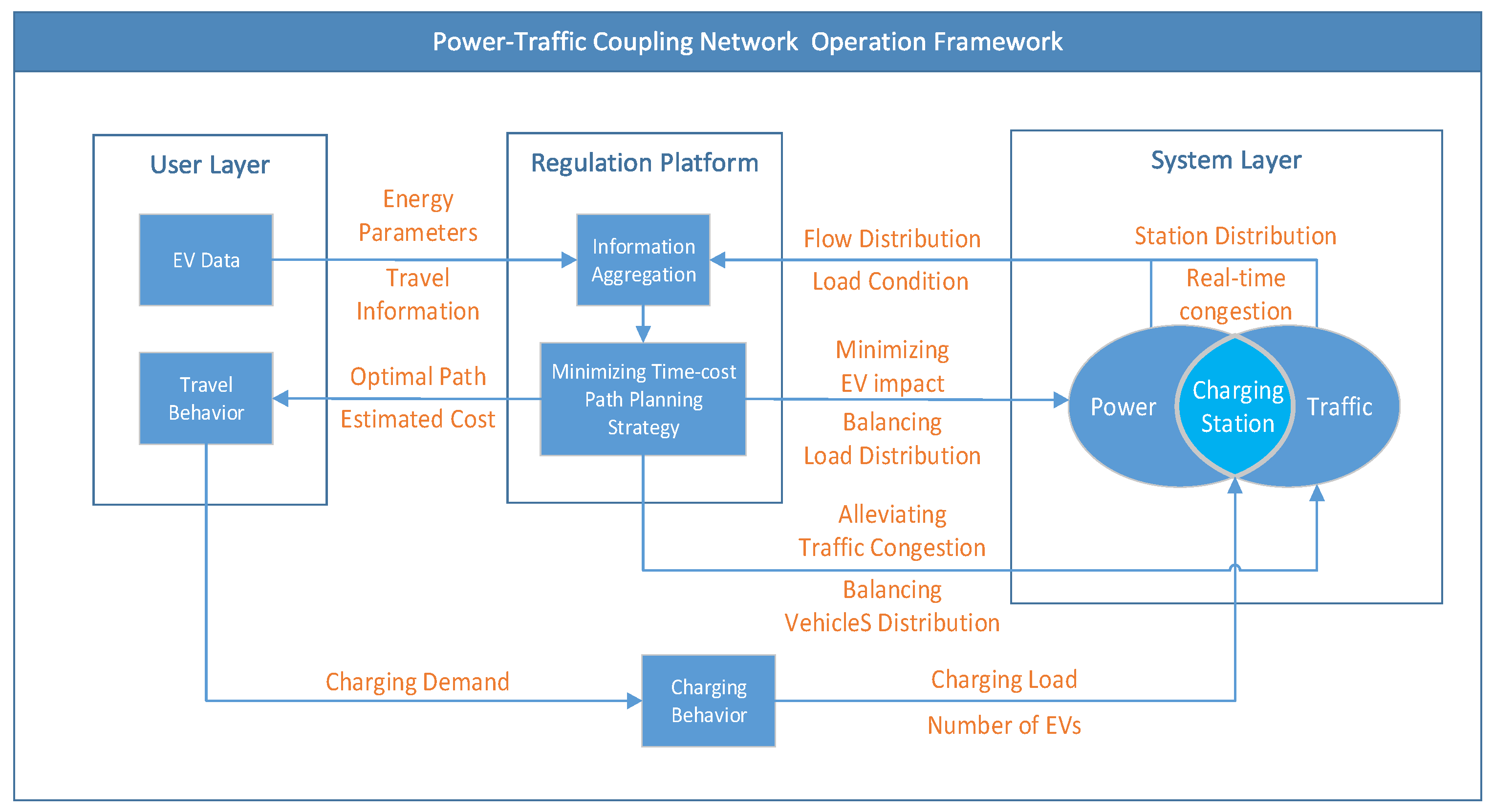
First, establish a coupled operation architecture between the power distribution network and the transportation network, as shown in Figure 5. In power–traffic coupling network, a simulation control platform is established to facilitate strategy deployment and interaction between entities, enabling the flow of information between the user layer and the system layer.
In the user layer, EV users participating in route planning provide the platform with vehicle battery parameters, travel time, O-D points, and other data. In the system layer, the power distribution network provides information on power flow distribution and load conditions at each node, while the transportation network provides information on road network geography and congestion levels at different time intervals. The control platform aggregates and calculates the received information to minimize user time costs. It then sends the optimal route planning results to the user layer, taking into account strategies that simultaneously reduce the impact of EVs on the power distribution network, alleviate traffic congestion caused by concentrated EV charging, and balance the spatial and temporal distribution of EV charging loads on the power distribution and transportation networks. Through platform information exchange and guidance on EV users’ travel and charging behaviors, the coupled operation of the power distribution network and transportation network is achieved.
The large-scale travel behavior of EVs directly affects the operation of the road network. Depending on the travel routes, the electricity consumption and charging behavior of EVs can change, thus simultaneously affecting traffic congestion levels and power grid flow. The rational planning of travel routes and mid-journey charging paths plays a crucial role in the coupled operation of the power distribution network and transportation network.
The most commonly used path planning algorithm is Dijkstra’s algorithm, which calculates the optimal path. However, the traditional Dijkstra’s algorithm is based on fixed road network data, and the calculated actual time cost and energy consumption may deviate from the actual driving conditions. In other words, the traditional Dijkstra’s algorithm is only suitable for static road networks where the limiting factors on vehicle movement, such as road length, do not change over time. It is suitable for path planning with the objective of finding the shortest distance in unguided scenarios.
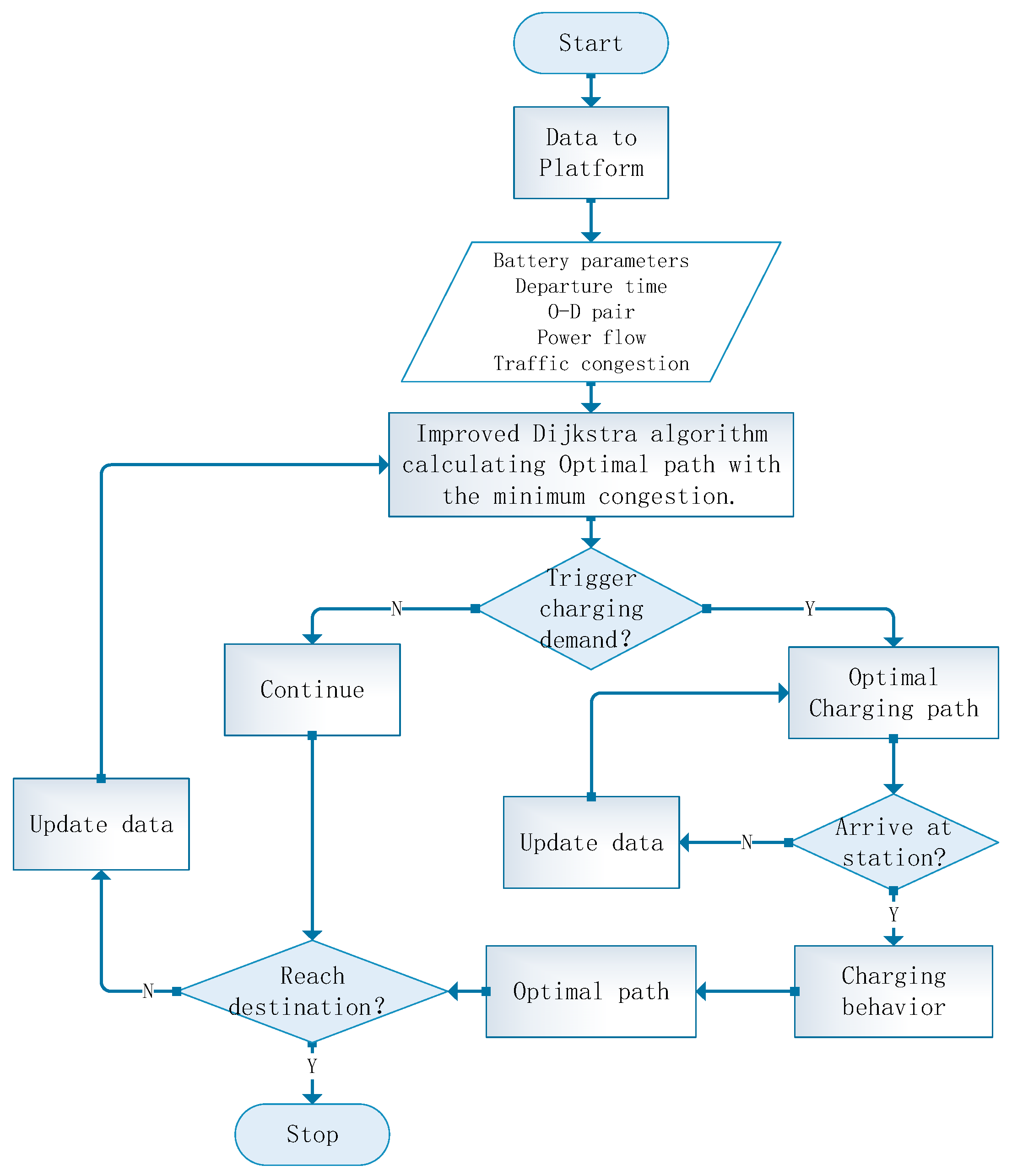
In the process of path traversal, the travel time and energy consumption of each road segment are related to the traffic flow at that moment. Considering the limitations of the traditional Dijkstra’s algorithm in time-guided scenarios, the improved planning process is as follows:
- Data collection: Collect EV’s departure time, OD points, battery level, as well as real-time operational data of the road network, such as traffic volume and congestion level.
- Cost calculation: Modify the cost calculation in the traditional Dijkstra’s algorithm by incorporating real-time road congestion data obtained from the road network. With this improvement, the algorithm no longer solely relies on static road segment lengths but also takes into account factors such as time and traffic conditions. This allows for a more accurate estimation of travel time and energy consumption.
- Dynamic routing: By utilizing the improved path planning algorithm, dynamic paths can be computed based on varying traffic conditions and EV parameters. Users can obtain the estimated travel time and energy consumption for the corresponding paths.
- Charging Station Selection: Incorporating the location and capacity of charging stations into the planning process. Solving for the optimal intermediate charging path based on the remaining battery charge and the availability of charging stations along the route.
- Iterative Optimization: Continuously updating traffic flow data and adjusting path planning algorithms according to real-time conditions to ensure that the planned path can accurately calculate the travel cost under changes in traffic and energy operations.
By introducing real-time data and dynamic path planning, the limitations of the traditional Dijkstra’s algorithm in time-guided scenarios have been addressed, providing EVs with more accurate and reasonable path planning.
The optimization objective is to minimize the user’s travel time cost (tct), which is represented by the sum of road impedance along the total path, including charging behaviors, to minimize time delays. It can be expressed as
The process of EV path planning based on the improved Dijkstra’s algorithm is shown in Figure 6.
5. Case Analysis
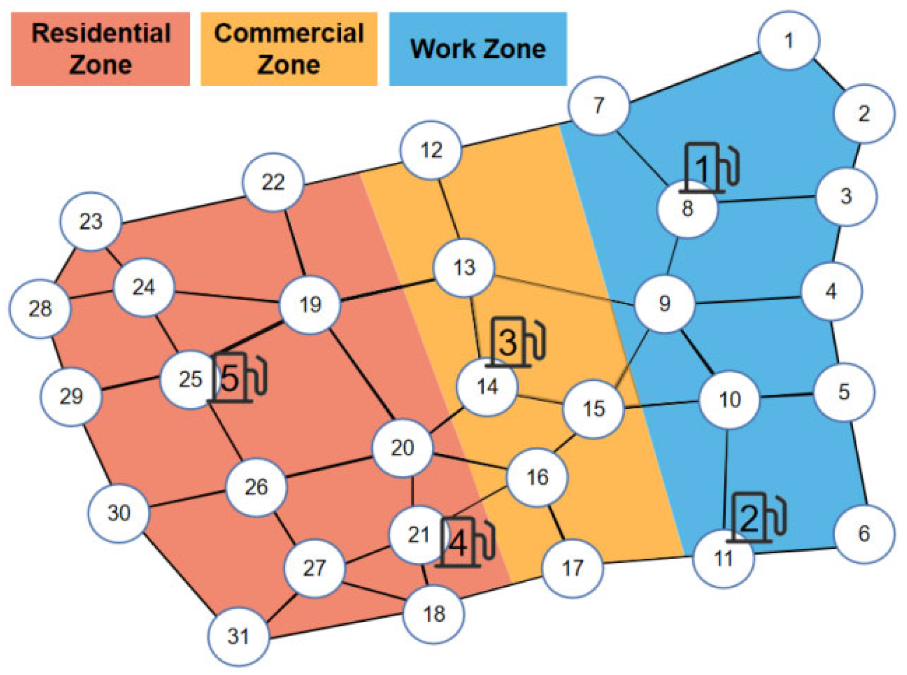
This article analyzes the operational situation of a typical working day in the road network of a certain area. As shown in Figure 7, the road network consists of 31 nodes and 52 roads. The area is divided into a working zone (W, including nodes 1–11), a commercial zone (C, including nodes 12–17), and a residential zone (R, including nodes 18–31). There are five charging stations located at nodes 8, 11, 14, 21, and 25, with two in the residential zone, two in the working zone, and one in the commercial zone.
This article sets a basic scale of 1000 EVs for the participating route planning, all of which are private cars. It assumes that the starting point of the first trip each day is in the residential area. Based on the survey data on the travel conditions of Chinese residents in the literature [31], three types of travel demands are set as shown in Table 1. The timing of EV travel mainly concentrates within the two time periods of morning and evening peaks. A charging demand is triggered when the real-time battery level falls below 0.3.
5.1. Simulation Results of Electric Vehicle Travel Behavior
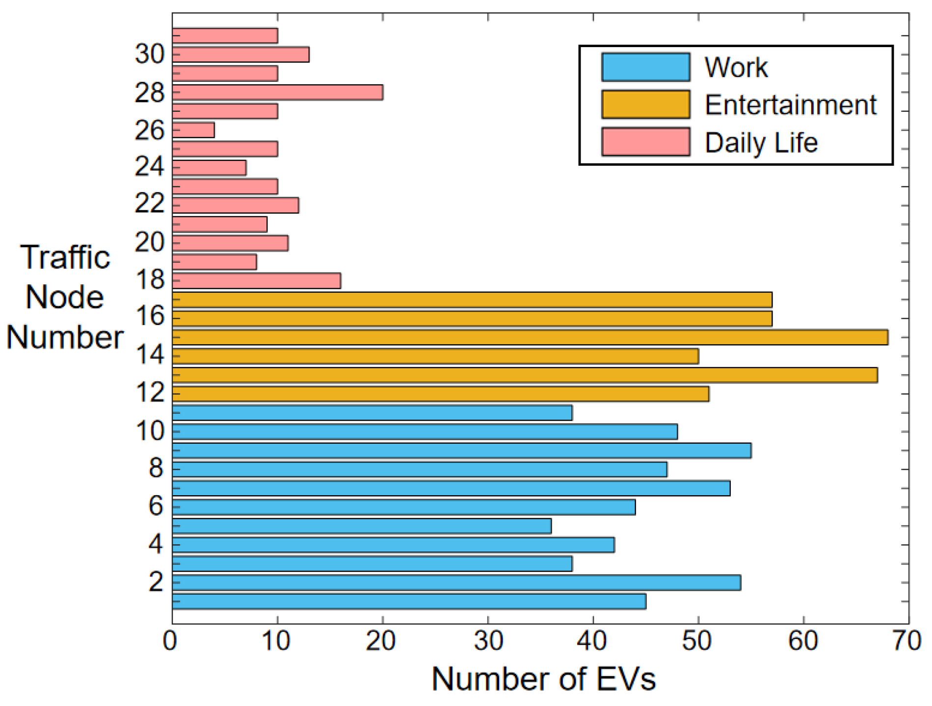
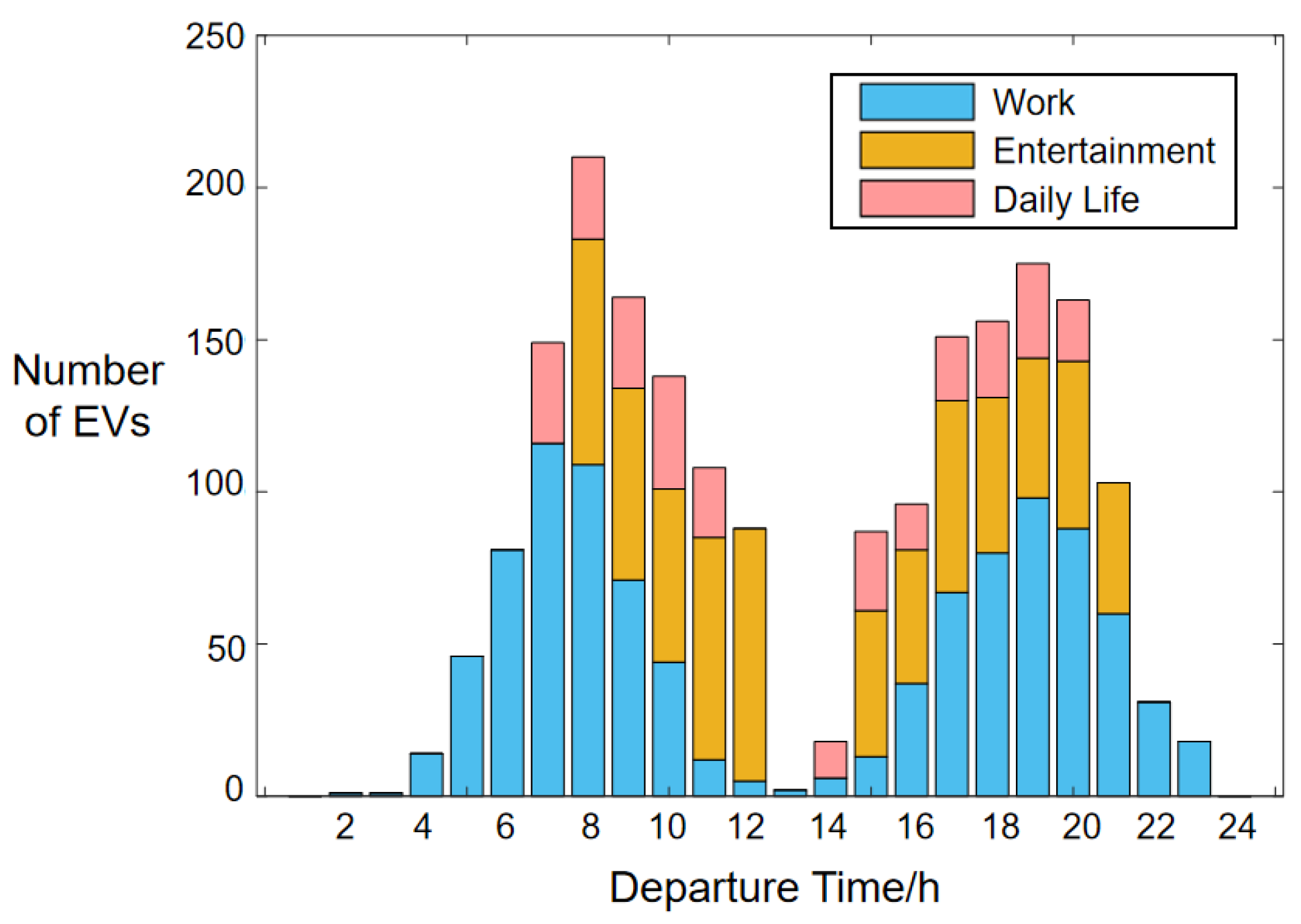
Based on the zoning of the road network and the different travel chains of EVs, taking the first travel segment, which is the outbound trip, as an example, all depart from the residential area. The basic travel characteristics of EVs are shown in Figure 8 and Figure 9.
According to the data from Figure 8, the number of vehicles traveling to the workplace is the highest, but the coverage area of the workplace is larger, as shown in Figure 7, resulting in relatively fewer vehicles in each node. On the other hand, vehicles traveling to commercial areas, although their proportion is slightly smaller, are concentrated in a smaller commercial area, resulting in a relatively larger number of vehicles. Additionally, commercial areas are often the necessary route for vehicles traveling to the workplace, making it more prone to traffic congestion. As depicted in Figure 9, EV travel exhibits clear morning and evening peak characteristics within a 24 h period.
5.2. Results of Electric Vehicles Route Planning Optimization
EV users who do not participate in route planning can only obtain direct information, such as the length of road segments, without access to real-time information on traffic congestion and travel time. Therefore, they choose the shortest distance route for travel. On the other hand, EV users who participate in guidance can interact with the power grid and road network to obtain real-time traffic information for different locations and time periods. Their goal is to plan travel routes with the shortest travel time, thus avoiding congested road sections.
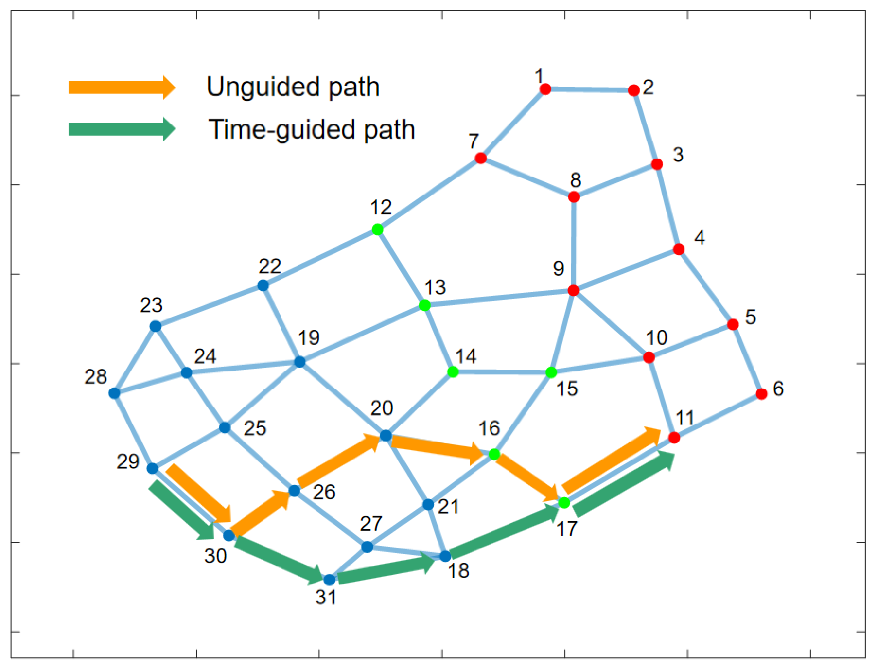
5.2.1. Electric Vehicle Travel Paths
Taking the first segment of the travel chain of vehicle 8, which does not trigger charging demand, as an example, the travel time is 6 am, and its O-D nodes are 29–11. As shown in Figure 10, the shortest distance travel route without guidance is (29–30–26–20–16–17–11). In the shortest travel time guidance path, based on real-time road congestion, the optimal travel path is (29–30–31–18–17–11).
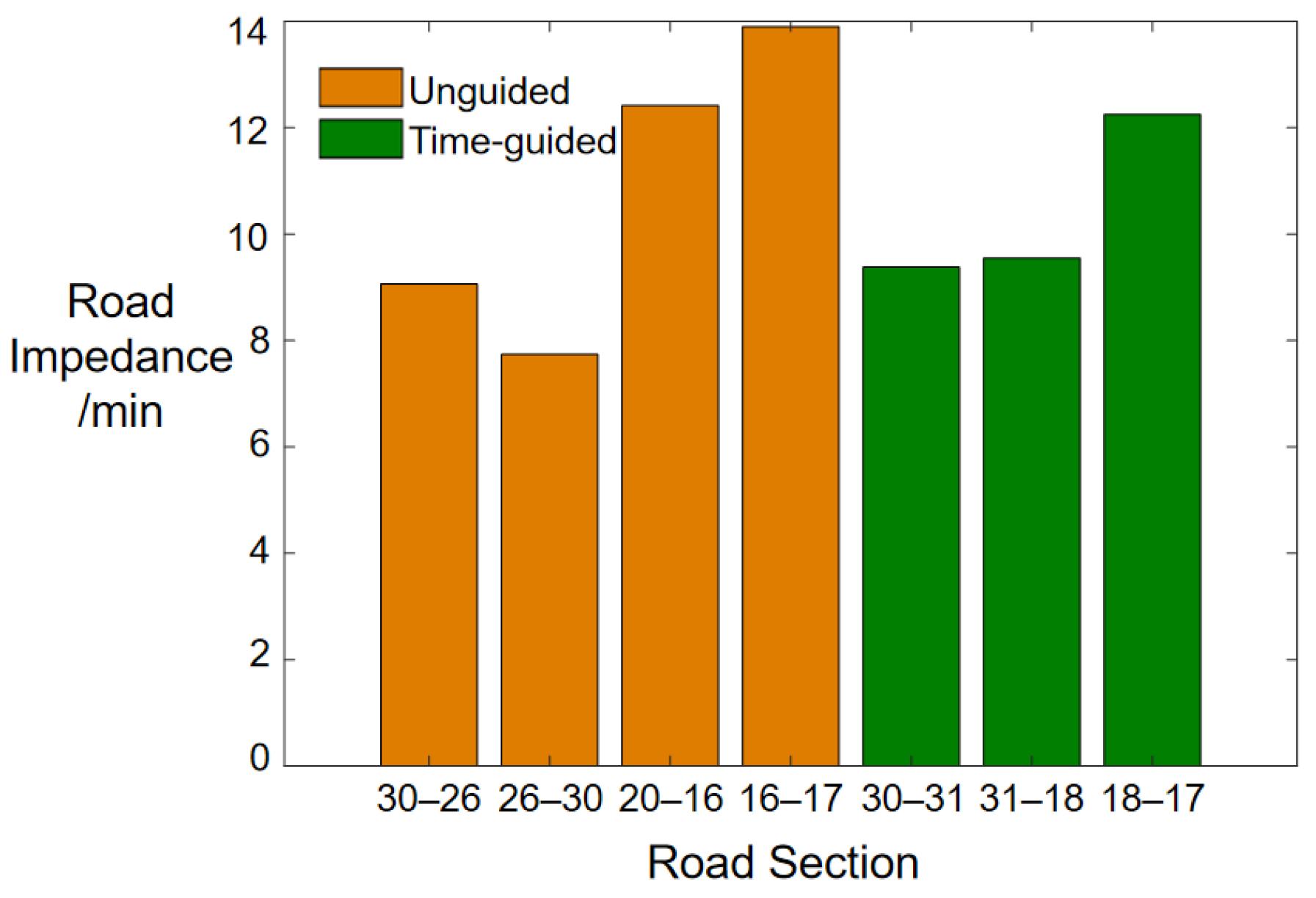
The road impedance data for the corresponding segments of the two paths are shown in Figure 11.
The segment of 30–26–20–16–17 has the same length as the segment of 30–31–18–17. However, the driving path guided by time avoids driving through relatively more congested residential areas and commercial districts, reducing the number of segments and decreasing the time cost for the driver by 18%. Additionally, the increased driving speed on this path reduces the energy consumption of the vehicle. The comparison is shown in Table 2.
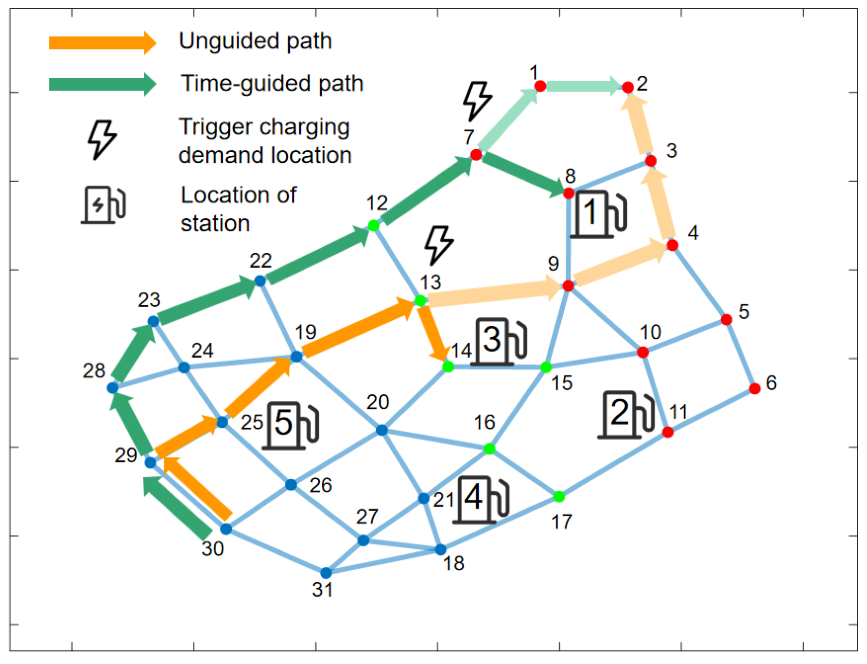
5.2.2. Electric Vehicle Midway Charging Paths
Taking vehicle 558, which triggered the charging demand, as an example, its O-D nodes are 30–2. As shown in Figure 12, in the absence of guidance, based on its initial path (30–29–25–19–13–9–4–3–2), when reaching node 13, the charging demand is triggered at 9 am. The vehicle owner then goes to the nearest charging station, which is station 3. The EV charging path is 13-14. As for vehicle 558, following the shortest time guidance, the initial path is (30–29–28–23–22–12–7–1–2). At 9 am, when reaching node 7, the charging demand is triggered. According to real-time road network data, the EV is guided to charging station 1, and the shortest time charging path is 7–8.
In the two scenarios, due to the different initial planned paths, the location where the EV triggers the charging demand is also different. Combining the distribution of charging stations within the road network, in the absence of guidance, the EV charging path chooses the nearest charging station, which is station 3 (node 14). However, it is located in the central business district, where the road sections are relatively congested, resulting in a longer charging travel time for the vehicle owner. Under the guidance of the shortest time, the EV selects charging station 1 (node 8), which is located in the working area. Although the charging travel distance is slightly longer, it saves travel time. At the same time, smoother road sections reduce the power consumption of the EV during the charging journey. The comparison between the two is shown in Table 3.
5.3. Analysis of the Impact on the Distribution Network Side
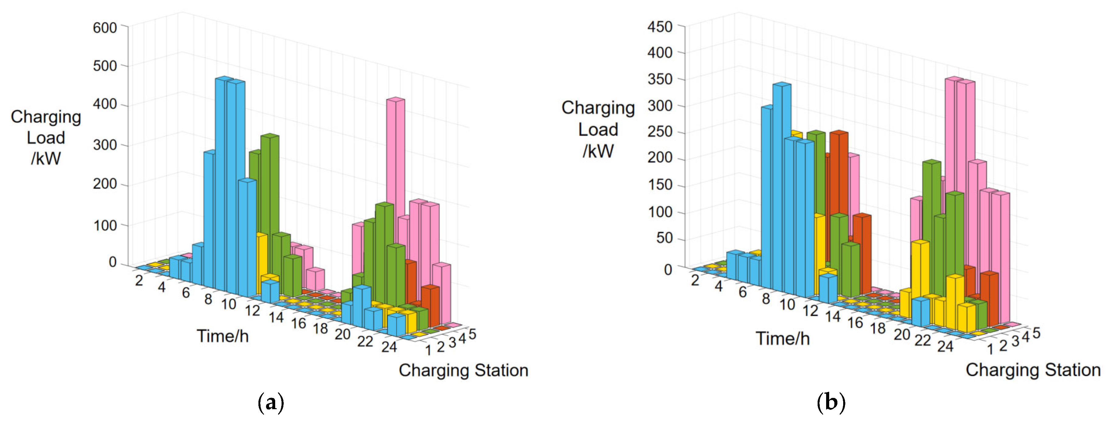
In the future energy society, it is essential for the power grid to maintain resiliency enhancement [32]. Due to the charging behavior of EVs, the charging load exhibits a bimodal characteristic, mainly concentrated in the morning peak hours (8–10 am) and evening peak hours (7–9 pm). During the morning peak hours, the charging load is mainly concentrated in the work area, such as charging station 1. During the evening peak hours, the charging load is concentrated in the residential area, such as charging station 5. This is because most of the charging demand comes from work vehicles, which are more likely to search for charging stations in commercial and work areas during their commute. When charging demand arises on the way back home, EVs are already closer to their destination, located in residential areas, leading to most of them accessing residential charging stations. The location of the charging stations in the power distribution network is indicated in Table 4.
The charging load in the two scenarios is shown in Figure 13a,b. In the unguided scenario, during the morning peak hours, a larger proportion of EVs prioritize work and entertainment needs. Based on their travel power consumption characteristics, these EVs tend to charge at stations 1 and 3, located within the working area and the central business district, respectively. During the evening peak hours, the vehicles return to residential areas, and station 5 is located at the center of the residential area. EVs that prioritize distance-based routes will choose station 5 for charging. This results in temporal and spatial imbalances in the load peaks, and the slow driving speed in congested areas leads to increased power consumption of EVs.
In the time-guided scenario, considering that the routes around high-load charging stations are more congested, leading to longer travel times, it can be observed that the charging load at high-load stations in the original unguided scenario is reduced, while the charging load at underutilized stations is increased. This overall balances the temporal and spatial distribution of the charging load, which is beneficial in reducing the pressure on power distribution networks.
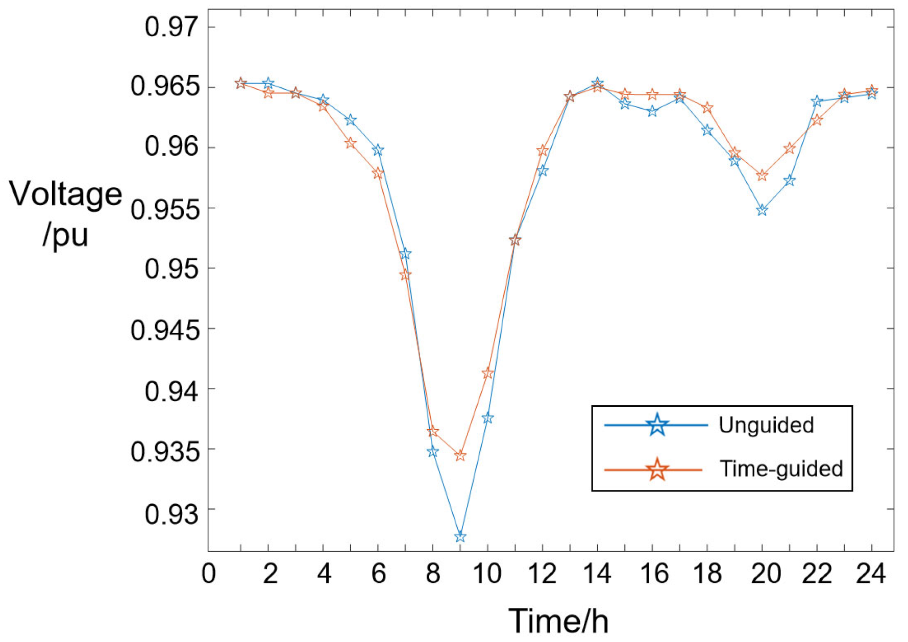
In Figure 14, in the scenario where the EV penetration rate is 35%, node 14 experiences a significant drop in voltage during two charging peak periods. In the early morning, at 9 o’clock, without guidance, the voltage drops to below 0.93, exceeding the safety operating requirement range (7% below the rated voltage). However, after implementing the time guidance strategy, the degree of voltage drop at node 14 is reduced, and the voltage is raised to 0.935, which is beneficial for the safe and stable operation of the power grid.
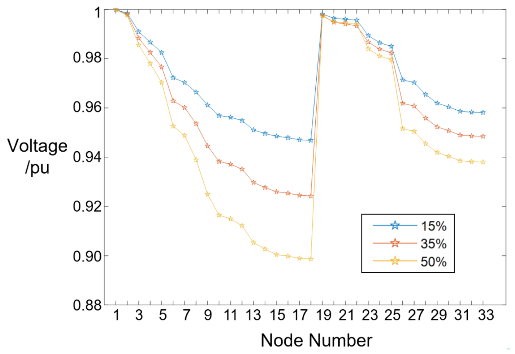
Figure 15 illustrates the voltage levels at different nodes at 8 am under varying EV penetration rates. Under 15% and 35% penetration rates, the voltage remains around 0.93, which is acceptable. However, when the penetration rate reaches 50%, some nodes experience voltages below 0.9, which can impact the safety of the power grid. This indicates that as the scale of EVs expands in the future, it will pose even more challenging demands on power grid operations.
5.4. Analysis of the Impacts on the Transportation Side
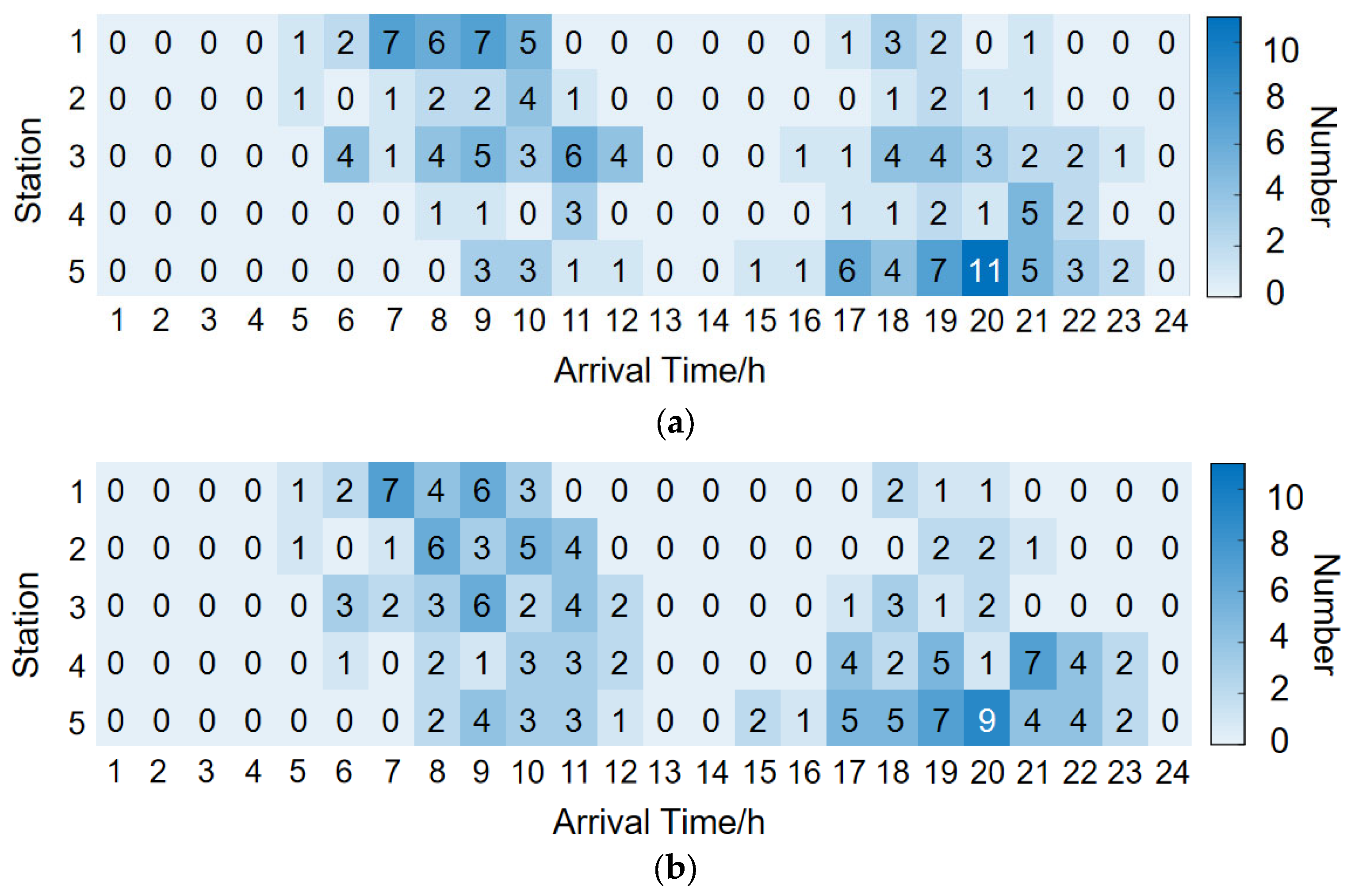
When EVs trigger the charging demand during the driving process, they will travel to the corresponding charging station along the optimal path based on the current location and the corresponding scenario. According to the study in reference [33], when a large number of EVs concentrate on charging, it will have an impact on the surrounding traffic conditions and exacerbate congestion near the charging stations. The number of vehicles accessing the charging station at different times of the day is shown in Figure 16a,b.
Looking at the two scenarios combined, EVs in both scenarios tend to gather at the charging stations during the morning and evening peak periods. In the morning, a large proportion of EVs with work-related demands drive to the work area and trigger the charging demand. EVs with entertainment demands and some work-related demands enter the commercial area for charging while charging stations in residential areas are more frequented by EVs driving within residential areas for daily-life demands. In the evening, as all EVs return to residential areas, charging vehicles are concentrated mostly in residential areas.
In the unguided scenario, as shown in Figure 16a, there is a significant difference in the number of vehicles entering each charging station, and the distribution is uneven. During the morning peak period, most of the charging vehicles are concentrated at stations 1 and 3, while during the evening peak period, they are mostly concentrated at station 5. This is because in the unguided paths, distance is prioritized, and charging stations located closer to the central areas of each region are chosen first to shorten the travel distance. This may lead to increased traffic congestion around the charging stations.
Comparing the unguided scenario with the time-guided scenario, as shown in Figure 16b, it can be seen that, especially during the morning peak period, the distribution of charging vehicles is more balanced. Due to the higher congestion levels in the central areas of each region, especially in the commercial area, the vehicles that were originally charging at stations 1 and 3 are guided to stations 2, 4, and 5, located near the smooth traffic sections. During the evening peak period, all private vehicles return to residential areas, and in the time-guided scenario, EVs still gather in residential areas for charging. However, compared to before, some EVs that were originally concentrated at station 5 are guided to station 4. The number of charging vehicles in residential areas is clearly shared between stations 4 and 5, alleviating the extra congestion caused by excessive concentration of EVs at a single charging station. In other words, in the time-guided scenario, while saving user’s time costs, the distribution of vehicles between charging stations is balanced, and traffic congestion is alleviated.
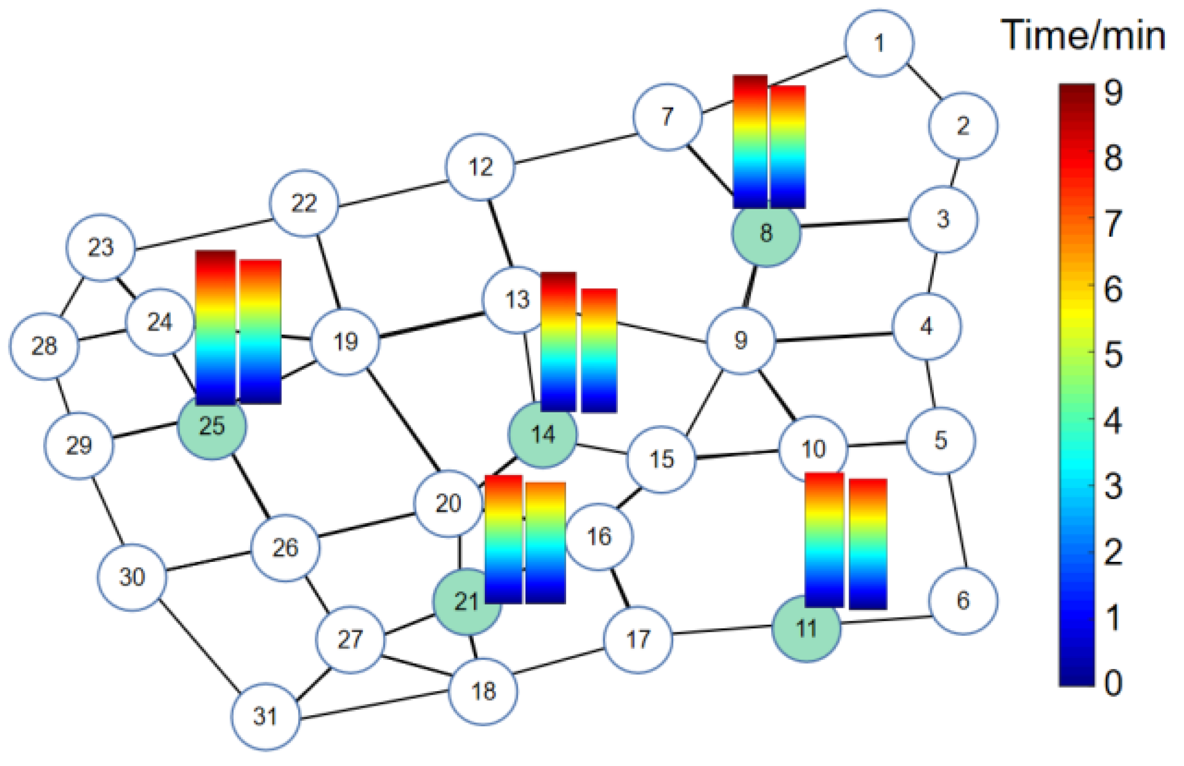
To quantify the alleviation of traffic congestion by EV route planning in the time-guided scenario, we can refer to Figure 17. We selected 9 am during the peak period and combined it with real-time congestion information of the roads around each charging station to obtain the average road impedance. The heat columns on the charging station nodes represent the average road impedance around them. The left side represents the unguided scenario, while the right side represents the time-guided scenario. By comparing the two, we can observe that the time-guided scenario, guided by the shortest travel time, changes the charging time period for EVs, avoiding concentrated charging during peak hours. This significantly reduces the travel time on the roads near the charging stations, thereby alleviating the level of traffic congestion.
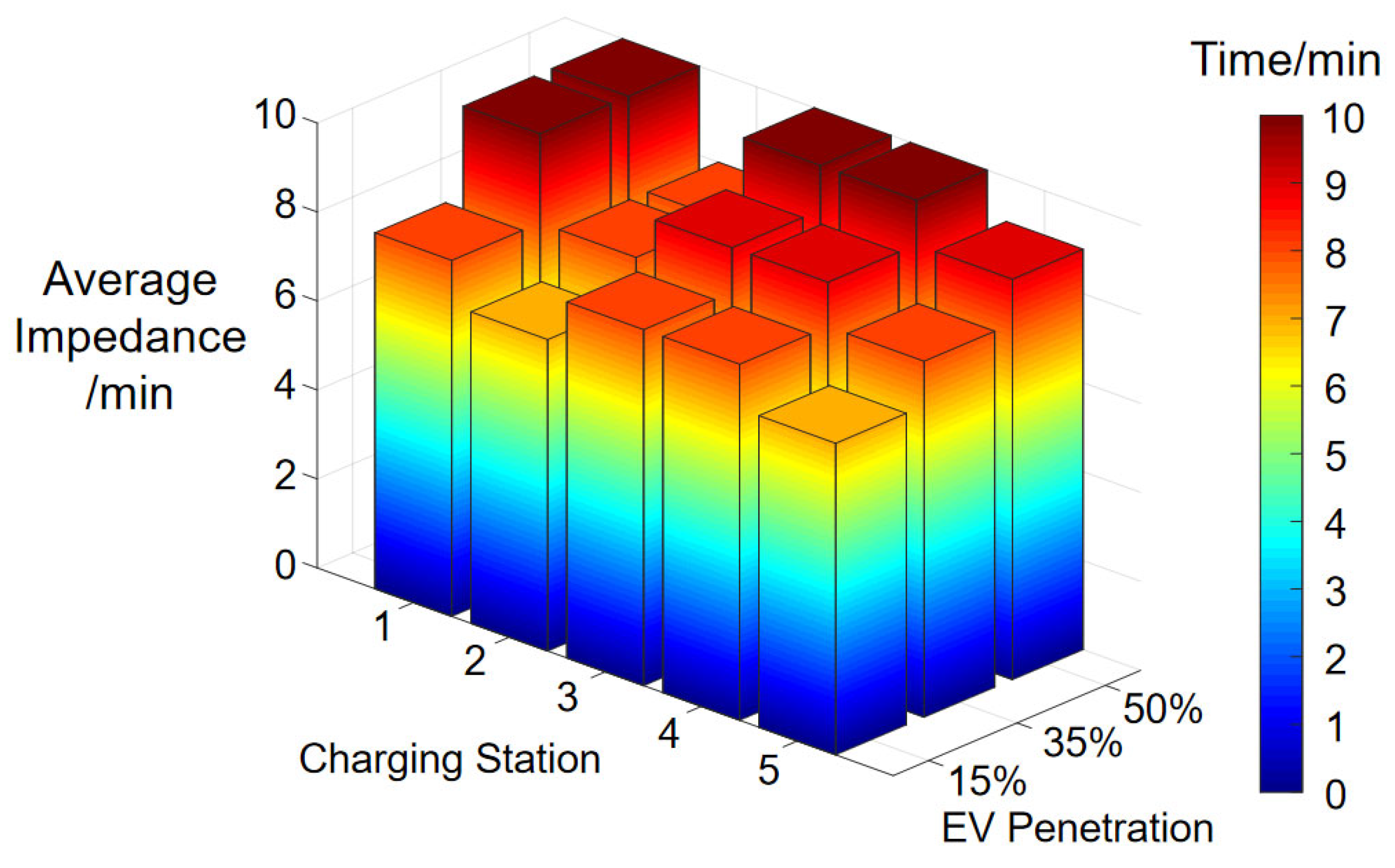
As the penetration rate of EVs increases, the road impedance around charging stations also changes. Taking the peak charging time at 9 am as an example, the average road impedance around each station is shown in Figure 18. It can be seen that with the increase in EV penetration rate, the road impedance near charging stations also increases, resulting in more congested traffic. In the future, with the large-scale development of EVs, the user’s time cost will also be greatly affected.
6. Conclusions
This paper takes into account that the driving behavior of EVs is greatly influenced by road travel time and utilizes it to guide EV routing. A real-time road network and road impedance model based on graph theory methods are established to describe the spatiotemporal characteristics of EVs. The EV travel chains are classified based on the distribution of the road network regions, and EV routing is planned using Dijkstra’s shortest path algorithm. The results show that
- Compared to the shortest distance path without guidance, the EV path under the traffic impedance guidance strategy in this paper can significantly reduce the travel energy consumption and time cost by approximately 18% with only a small increase in distance cost. This can be applied in subsequent research on improving user travel planning satisfaction.
- The strategy proposed in this paper can achieve a more balanced spatio-temporal distribution of charging load to alleviate the pressure on the regional power grid. This method can improve the degree of voltage drop in the power grid caused by EV charging behavior within the safety requirement of 7%. By analyzing different levels of EV penetration, it is evident that the future significant increase in EV penetration will pose greater challenges to grid operations. The research findings of this paper will provide a basis for addressing these risks.
- The guiding strategy presented in this paper can achieve a more balanced spatio-temporal distribution of vehicles triggering charging demands while reducing road congestion around charging stations and alleviating traffic congestion. With the continuous rapid growth in the number of EVs in the future, it will also bring various impacts to the transportation system. The findings of this paper can serve as one of the fundamental methods to mitigate adverse effects such as traffic congestion.
This study still has some limitations, such as the characterization of user costs only considering time and energy costs and insufficient emphasis on the load characteristics of EV users in different regions. To address the aforementioned issues, in future research, we will conduct a study on differentiated user characteristics and incorporate charging station service fees, among other factors, to perform comprehensive cost calculations that include users’ economic costs.
Author Contributions
Conceptualization, J.L. and S.T.; methodology, J.L. and Z.W.; software, S.T.; validation, J.L. and S.T.; formal analysis, S.T.; investigation, N.Z.; resources, G.L.; data curation, J.L.; writing—original draft preparation, S.T.; writing—review and editing, W.L., J.L. and Z.W.; visualization, J.L. and G.L.; supervision, Z.W. and N.Z.; project administration, J.L. and S.T.; funding acquisition, W.L. All authors have read and agreed to the published version of the manuscript.
Funding
This research was funded by the Jiebangguashuai project of Inner Mongolia, grant number 2022JBGS0043.
Institutional Review Board Statement
Not applicable.
Informed Consent Statement
Not applicable.
Data Availability Statement
The data presented in this study are available through request to the corresponding author.
Conflicts of Interest
The authors declare no conflict of interest.
References
- Alanazi, F. Electric Vehicles: Benefits, Challenges, and Potential Solutions for Widespread Adaptation. Appl. Sci. 2023, 13, 6016. [Google Scholar] [CrossRef]
- Wu, Z.; Zhou, M.; Zhang, Z.; Zhao, H.; Wang, J.; Xu, J.; Li, G. An incentive profit-sharing mechanism for welfare transfer in balancing market integration. Renew. Sustain. Energy Rev. 2022, 168, 112762. [Google Scholar] [CrossRef]
- General Office of the State Council of the People’s Republic of China. Development Plan for the New Energy Vehicle Industry (2021–2035); General Office of the State Council of the People’s Republic of China: Beijing, China, 2020.
- Chang, X.; Wu, Z.; Wang, J.; Zhang, X.; Zhou, M.; Yu, T.; Wang, Y. The coupling effect of carbon emission trading and tradable green certificates under electricity marketization in China. Renew. Sustain. Energy Rev. 2023, 187, 113750. [Google Scholar] [CrossRef]
- Tang, D.; Wang, P. Nodal Impact Assessment and Alleviation of Moving Electric Vehicle Loads: From Traffic Flow to Power Flow. IEEE Trans. Power Syst. 2016, 31, 4231–4242. [Google Scholar] [CrossRef]
- Li, J.; Shi, Y.; Zhang, L.; Yang, X.; Wang, L.; Chen, X. Optimization strategy for the energy storage capacity of a charging station with photovoltaic and energy storage considering orderly charging of electric vehicles. Power Syst. Prot. Control 2021, 49, 94–102. [Google Scholar]
- Deželak, K.; Sredenšek, K.; Seme, S. Energy Consumption and Grid Interaction Analysis of Electric Vehicles Based on Particle Swarm Optimisation Method. Energies 2023, 16, 5393. [Google Scholar] [CrossRef]
- Chen, L.; Nie, Y.; Zhong, Q. A Model for Electric Vehicle Charging Load Forecasting Based on Trip Chains. Trans. China Electrotech. Soc. 2015, 30, 216–225. [Google Scholar]
- Zhang, H.; Hu, Z.; Song, Y.; Xu, Z.; Jia, L. A Prediction Method for Electric Vehicle Charging Load Considering Spatial and Temporal Distribution. Autom. Electr. Power Syst. 2014, 38, 13–20. [Google Scholar]
- Tayarani, H.; Jahangir, H.; Nadafianshahamabadi, R.; Aliakbar Golkar, M.; Ahmadian, A.; Elkamel, A. Optimal Charging of Plug-In Electric Vehicle: Considering Travel Behavior Uncertainties and Battery Degradation. Appl. Sci. 2019, 9, 3420. [Google Scholar] [CrossRef]
- Cannavacciuolo, G.; Maino, C.; Misul, D.A.; Spessa, E. A Model for the Estimation of the Residual Driving Range of Battery Electric Vehicles Including Battery Ageing, Thermal Effects and Auxiliaries. Appl. Sci. 2021, 11, 9316. [Google Scholar] [CrossRef]
- Cheng, S.; Zhong, S.; Shang, D.; Wei, K.; Wang, C. Dynamic reconfiguration of an active distribution network considering temporal and spatial load distribution characteristics of electric vehicles. Power Syst. Prot. Control 2022, 50, 1–13. [Google Scholar]
- Shao, Y.; Mu, Y.; Yu, X.; Dong, X.; Jia, H. A Spatial-temporal Charging Load Forecast and Impact Analysis Method for Distribution Network Using EVs-Traffic-Distribution Model. Proc. CSEE 2017, 37, 5207–5219. [Google Scholar]
- Zhang, C.; Peng, K.; Xiao, C.; Zhang, X.; Xing, L. EV charging guiding strategy based on coordination of EVs-road-network. Electr. Power Autom. Equip. 2022, 42, 125–133. [Google Scholar]
- Zheng, Y.; Li, F.; Dong, J.; Luo, J.; Zhang, M. Optimal Dispatch Strategy of Spatio-Temporal Flexibility for Electric Vehicle Charging and Discharging in Vehicle-Road-Grid Mode. Autom. Electr. Power Syst. 2022, 46, 88–97. [Google Scholar]
- Wang, H.; Leng, X.; Pan, Y.; Bian, J.; Yu, Z. Orderly charging and discharging strategy of electric vehicle considering spatio-temporal characteristic and time cost. Electr. Power Autom. Equip. 2022, 42, 86–91. [Google Scholar]
- Bachiri, K.; Yahyaouy, A.; Gualous, H.; Malek, M.; Bennani, Y.; Makany, P.; Rogovschi, N. Multi-Agent DDPG Based Electric Vehicles Charging Station Recommendation. Energies 2023, 16, 6067. [Google Scholar] [CrossRef]
- Yang, W.; Liu, W.; Chung, C.Y.; Wen, F. Joint planning of EV fast charging stations and power distribution systems with balanced traffic flow assignment. IEEE Trans. Ind. Inform. 2020, 17, 1795–1809. [Google Scholar] [CrossRef]
- Yuan, H.; Zhang, J.; Xu, P.; Fang, Z. Fast Charging Demand Guidance in Coupled Power-Transportation Networks Based on Graph Reinforcement Learning. Power Syst. Technol. 2021, 45, 979–986. [Google Scholar]
- Tang, Q.; Li, D.; Zhang, Y.; Chen, X. Dynamic Path-Planning and Charging Optimization for Autonomous Electric Vehicles in Transportation Networks. Appl. Sci. 2023, 13, 5476. [Google Scholar] [CrossRef]
- Ahsini, Y.; Díaz-Masa, P.; Inglés, B.; Rubio, A.; Martínez, A.; Magraner, A.; Conejero, J.A. The Electric Vehicle Traveling Salesman Problem on Digital Elevation Models for Traffic-Aware Urban Logistics. Algorithms 2023, 16, 402. [Google Scholar] [CrossRef]
- Luo, Y.; Zhu, T.; Wan, S.; Zhang, S.; Li, K. Optimal charging scheduling for large-scale EV (electric vehicle) deployment based on the interaction of the smart-grid and intelligent-transport systems. Energy 2016, 97, 359–368. [Google Scholar] [CrossRef]
- Chen, S. Research on Practical Velocity-Volume Model of Urban Streets. Master’s Thesis, Southeast University, Nanjing, China, 2004. [Google Scholar]
- Yu, T. Study of Optimal Path in Traffic Network with Random Link Travel Times Based on Real-Time Traffic Information. Master’s Thesis, Nanjing Forestry University, Nanjing, China, 2017. [Google Scholar]
- Wu, Z.; Wang, J.; Zhong, H.; Gao, F.; Pu, T.; Tan, C.; Chen, X.; Li, G.; Zhao, H.; Zhou, M.; et al. Sharing Economy in Local Energy Markets. J. Mod. Power Syst. Clean Energy 2023, 11, 714–726. [Google Scholar] [CrossRef]
- Mu, Y.; Wu, J.; Jenkins, N.; Jia, H.; Wang, C. A spatial–temporal model for grid impact analysis of plug-in electric vehicles. Appl. Energy 2014, 114, 456–465. [Google Scholar] [CrossRef]
- Xing, Q.; Chen, Z.; Zhang, Z.; Xu, X.; Zhang, T.; Huang, X.; Wang, H. Urban Electric Vehicle Fast-Charging Demand Forecasting Model Based on Data-Driven Approach and Human Decision-Making Behavior. Energies 2020, 13, 1412. [Google Scholar] [CrossRef]
- Song, Y. Energy Consumption Modeling and Cruising Range Estimation Based on Driving Cycle for Electric Vehicles. Master’s Thesis, Beijing Jiaotong University, Beijing, China, 2014. [Google Scholar]
- Federal Highway Administration. 2017 National Household Travel Survey; Federal Highway Administration: Washington, DC, USA, 2018.
- Zhang, L.; Xu, C.; Wang, L.; Li, J.; Chen, X.; Yang, X.; Shi, Y. OD matrix based spatiotemporal distribution of EV charging load prediction. Power Syst. Prot. Control 2021, 49, 82–91. [Google Scholar]
- Baidu Map. China Urban Transportation Report. 2018. Available online: https://huiyan.baidu.com/cms/report/2018annualtrafficreport/index.html (accessed on 18 June 2023).
- Wu, Z.; Wang, J.; Zhou, M.; Xia, Q.; Tan, C.-W.; Li, G. Incentivizing Frequency Provision of Power-to-Hydrogen Toward Grid Resiliency Enhancement. IEEE Trans. Ind. Inform. 2023, 19, 9370–9381. [Google Scholar] [CrossRef]
- Ji, Z.; Huang, X. Plug-in electric vehicle charging infrastructure deployment of China towards 2020: Policies, methodologies, and challenges. Renew. Sustain. Energy Rev. 2018, 90, 710–727. [Google Scholar] [CrossRef]
Figure 1.
Coupled network of the distribution grid, EVs, and the transportation network.

Figure 2.
Topological structure of the traffic road network.

Figure 3.
Illustration of road impedance.

Figure 4.
Schematic diagram of road network area division.

Figure 5.
Power–traffic coupling network operation framework.

Figure 6.
Process of EV driving path planning.

Figure 7.
Distribution and zoning of the road network.

Figure 8.
Spatial distribution of EVs travel.

Figure 9.
Temporal distribution of EVs travel.

Figure 10.
Comparison of EV travel paths.

Figure 11.
Comparison of impedance levels along the route segments.

Figure 12.
Comparison of EV midway charging paths.

Figure 13.
Charging load in (a) unguided scenario and (b) time-guided scenario.

Figure 14.
Voltage levels in two different scenarios.

Figure 15.
Voltage levels at different nodes under varying EV penetration rates.

Figure 16.
Number of EVs in (a) unguided scenario and (b) time-guided scenario.

Figure 17.
Average road impedance around each charging station in two scenarios.

Figure 18.
Average road impedance around each charging station at different EV penetration rates.


Table 1.
Proportion of EVs with different travel demands.
| Travel Demand | Driving Areas | Proportion |
|---|---|---|
| work | R–W | 50% |
| entertainment | R–C | 35% |
| daily life | R–R | 15% |
Table 2.
Driving path comparison in two scenarios.
| Driving Path | Distance (km) | Time Cost (h) | Energy Consumption (kWh) | |
|---|---|---|---|---|
| Unguided | 29–30–26–20–16–17–11 | 35 | 1.10 | 9.74 |
| Time-guided | 29–30–31–18–17–11 | 36 | 0.90 | 9.53 |
| Difference | \ | +1 | −0.2 | −0.21 |
Table 3.
Comparison of midway charging paths in two scenarios.
| Triggering Location | Charging Path | Distance (km) | Time Cost (h) | Energy Consumption (kWh) | |
|---|---|---|---|---|---|
| Unguided | 13 | 13–14 | 6 | 0.21 | 1.09 |
| Time-guided | 7 | 7–8 | 7 | 0.17 | 0.97 |
| Difference | \ | \ | +1 | −0.04 | −0.12 |
Table 4.
Location of the charging station in the power distribution network.
| Area | W | C | R | ||
|---|---|---|---|---|---|
| Charging station | NO. 1 | NO. 2 | NO. 3 | NO. 4 | NO. 5 |
| Distribution network | Node 8 | Node 11 | Node 14 | Node 21 | Node 25 |
Disclaimer/Publisher’s Note: The statements, opinions and data contained in all publications are solely those of the individual author(s) and contributor(s) and not of MDPI and/or the editor(s). MDPI and/or the editor(s) disclaim responsibility for any injury to people or property resulting from any ideas, methods, instructions or products referred to in the content. |
© 2023 by the authors. Licensee MDPI, Basel, Switzerland. This article is an open access article distributed under the terms and conditions of the Creative Commons Attribution (CC BY) license (https://creativecommons.org/licenses/by/4.0/).
Share and Cite
MDPI and ACS Style
Li, J.; Tian, S.; Zhang, N.; Liu, G.; Wu, Z.; Li, W. Optimization Strategy for Electric Vehicle Routing under Traffic Impedance Guidance. Appl. Sci. 2023, 13, 11474. https://doi.org/10.3390/app132011474
AMA Style
Li J, Tian S, Zhang N, Liu G, Wu Z, Li W. Optimization Strategy for Electric Vehicle Routing under Traffic Impedance Guidance. Applied Sciences. 2023; 13(20):11474. https://doi.org/10.3390/app132011474
Chicago/Turabian StyleLi, Jingyu, Shiyuan Tian, Na Zhang, Guangchen Liu, Zhaoyuan Wu, and Wenyi Li. 2023. "Optimization Strategy for Electric Vehicle Routing under Traffic Impedance Guidance" Applied Sciences 13, no. 20: 11474. https://doi.org/10.3390/app132011474
Note that from the first issue of 2016, this journal uses article numbers instead of page numbers. See further details here.