Creative Coding in Blender 2.92: A Primer

Jeremy Behreandt

·

Follow

30 min read

·

May 25, 2021

--

11

Listen

Share

This tutorial’s aim is to encourage creative coders to try Blender as a platform for procedural artwork. Blender is free software in the sense that no payment is required to download and use it. Furthermore, its source code is available online.

This is written for readers with some experience creative coding who wish to expand their toolset. We’ll write some Python scripts to animate geometry, add modifiers and constraints, create materials with Open Shading Language (OSL), and end with a glimpse at Blender’s grease pencil.

This tutorial was written with Blender version 2.92.

It is an update of an older tutorial written 3 years ago for Blender 2.79. Blender evolves rapidly. Its user interface and API change just as fast. If the scripts below raise errors, please check the change log to see if the API has changed since the script was written.

Configure Blender for Scripting

Unlike environments devoted solely to coding, Blender is a Swiss Army Knife. Animators, sculptors and texture artists will configure Blender differently to suit their workflow. For any given task, there are multiple ways to do it — whether by hotkey, menu, modifier, nodes and noodles, mouse click or script. The tips laid out in this section are not necessary, but will improve quality of life once we’re in the thick of Python scripting.

Read The Manual

Blender’s manual and scripting API can both be downloaded from the Internet. This enables us to bookmark local copies of each in our browser of choice, then continue coding even when offline.

System Console

When debugging a script, if we wish to read the diagnostic info returned from print commands, we can navigate to the menu bar, open Window, then click Toggle System Console.

This is also where error messages will inform us of why our script didn’t run.

Alternatively, we can open Blender from the command line.

Editor Layout

Blender allows us to swap editor panels by selecting from the drop-down menus in the top-left corner of each.

The drop-down menu is organized into categories; three editors fall under the Scripting category: Text Editor, Python Console and Info.

The info editor provides a history of editor transactions. It is helpful when we begin scripting because we can copy and paste an operation from the editor into a script (there is a drawback to this aproach that we’ll discuss later).

The console editor is interactive, which allows us to draft mathematical operations and use auto-complete to find appropriate fields and methods.

The scripting preset is one of many layout presets on the top menu bar to the right of the drop down menus. This preset includes the 3D view, interactive console, info, text editor, outliner and properties editor.

Keypresses are interpreted dependent on which editor the mouse cursor is hovering over. For this reason, it’s not recommended to use the text editor for more than reloading and running a script.

A white question mark inside a circle will appear in a red button when the script has been modified externally the conflict needs resolution.

Visual Studio Code is a good alternative to the text editor; for Python, VS Code benefits from Anaconda.

Visual Diagnostic Aides

The Preferences editor can be found in the Edit menu. Under the Interface tab, we check Python Tooltips. This will give us information about the method name called when we click a button.

If we’re interested in working with meshes primarily, we may also want to tick the check box that enables Developer Extras. This will give us a menu option in the 3D view overlays menu which displays vertex, edge and face indices.

However, for meshes with a lot of faces, be sure to turn this overlay off before entering edit mode.

We can also change the outliner editor’s display mode to show data in a way that more closely aligns with its code representation.

Hotkeys

Hotkeys can be reviewed and changed in Preferences.

For example, the default hotkey to run a script is Alt P. Again, this assumes the mouse is located over the text editor. In the 3D VIew, Alt P will open the clear parent menu.

While here, check to see that the interactive console’s autocomplete feature is set to your preference.

Add-Ons

Last but not least. We may code for education or for pleasure, but if we’re looking to achieve a certain effect, we can check the add-ons menu. More are available at online marketplaces. Not only do add-ons spare us from reinventing the wheel, if we look at their source code we may also gather insights into how to craft future scripts.

Python Syntax

As with any software that allows the user to create custom scripts, we must simultaneously learn a specific API and the programming language on which it relies. As with Processing and Java, Aseprite and Lua, Unity and C#, or Three and JavaScript, the more we know about the language the faster and more effectively we can use the API.

When translating our scripting work into Python, there are a few syntactic qualities to watch out for. We’ll highlight a few which may trip up coders hailing from other languages:

• Linebreaks conclude statements, not semi-colons.
• Blocks of code begin with a colon, :, and are offset by indentation. They are not enclosed by curly braces { and }.
• A data type is not specified when declaring a new variable.
• Comments are initiated with a hash-tag #, not double forward slash //.
• Booleans are True or False.
• Use or for ||, and for &&, not for !.
• An unassigned reference is None, not null or nil.
• // denotes floor division. This is not the same as integer division. -5 // 2 yields -3 while 5 // 2 yields 2.
• % denotes floor modulo, not truncation modulo. This is unlike C#, Java or JavaScript. -5 % 4 yields 3; 5 % 4 yields 1.
• Python includes an exponentiation operator, **. The circumflex, ^, is reserved for bitwise exclusive-or (XOR).
• Regarding abbreviations and capitalization: elif is used, not else if or elseif.
• Lists are initiated with square brackets , []; dictionaries, with curly braces, {}; tuples, with parentheses, ().
• Subscripts begin at 0, not 1. Negative indices are acceptable: -1 returns the last element.
• Python supports operator overloading, meaning operators can be used with objects from Blender’s mathutils module.

Beyond syntax is the “Pythonic idiom,” a style of coding in Python which promotes readability using features unique to the language; an example of idiomatic code would be the use of list comprehensions. This tutorial avoids Pythonic idiom where possible to make scripts easier to interpret in relation to other programming languages.

For more, see Python’s documentation.

Static Composition

Now that we’re oriented, let’s make some geometry.

Cartesian Grid

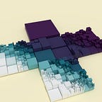
We begin with a grid of cubes. This exercise will acclimate us to Blender’s world coordinates, where positive z axis is up and positive y axis is forward.

To work with for loops, we make a range, then test whether an index is in that range. Python allows for named parameters in function calls, and Blender may require them in certain methods.

We separate a cube’s abstract location within the grid from its location in world coordinates. For example, a cube may be in the 2nd row, 3rd column and 7th layer of the grid, but be located at (50.0, 25.0, 100.0) in the scene, depending on the grid’s translation, rotation and scale.

In this case, we convert between real world and abstract coordinates by converting abstract location to a percent, adding the real world range’s lower bound, -extents, then multiplying by the range’s upper bound minus its lower bound, extents-(-extents) or extents * 2.

Editing the translation, rotation and scale of an object is distinguished in Blender from the transformations of vertices, faces and edges of which it is composed. We’ll create separate objects for now, but a single object with separate cubes in its mesh data is an alternative.

When we run this script, we should check how much time it takes to complete. The benefit of using bpy.ops methods is that they ease the transition from Blender’s GUI to scripting. The disadvantage is that they incur alot of overhead. Blender’s documentation offers the following advice: sample the system time at the beginning of the script, take another sample at the end of the script, then find the absolute difference between the two.

To address this issue, let’s refactor. To do so, we need the bmesh module. This provies tools for more direct mesh creation. Another tutorial covers this module in greater depth, so we’ll not do so here.

Cartesian Grid, Refactored

Additionally, we’ll flatten the three nested for loops into one. This is a generalization of the usual technique to convert from an index to a coordinate: x = i % width, y = i // width.

For the ground, we call create_grid instead of create_cube. For lights, we call bpy.data.lights.new; for a camera, bpy.data.cameras.new. After this, we’ll omit this from code snippets and assume that ground, camera and lights can be appended if desired. The general workflow, though, deserves comment: new information is created in bpy.data, it is then appended to a collection in a context.

Were we to assume that a given cube’s vertices, edges or faces won’t change in the future, we could optimize further by creating only one mesh data from a BMesh. Then, all objects could refer to the same data. This is called instancing.

Materials are assigned to data by default, so we’d need other techniques — not yet introduced — to give each cube a different color. For example, we could assign to the object’s color. We’d then create one material, ensure nodes are enabled, then use an Object Info Node to pass on the color data to the Principled BSDF.

The gamma in our colors is adjusted by raising them to a power of 2.2.

Sidebar: Color

Color is too complex a topic to provide adequate treatment here. However, we can’t avoid the topic either. In short, Blender uses a color management system. There are several debates on Blender Stack Exchange and Blender Artists around issues with its implementation. It can be found in the Properties Editor under Render properties.

A color we observe in Blender may appear to be the same as a color in another context, but have different numerical values. Conversely, a color may look different in Blender, yet have the same numerical values. Confusing the matter further is how Blender’s color picker displays hexadecimal values such as #AABBCC relative to color channels in the range [0.0, 1.0].

We can test this by looking at a middle cube in a given row, column or layer of the cube grid above. Let’s look at a magenta-purple that develops along the x axis at the top — z positive — edge of the grid.

For the moment, set aside debate over whether 128 or 127 is the “middle,” and whether we convert to [0.0, 1.0] with division by 255.0 or 256.0. The color picker’s hexadecimal value #8000FF corresponds to (0.218, 0.0, 1.0), not 128.0 / 255.0 or 0.501961 as we might expect. The hexadecimal #DE00FF corresponds to the RGB values (0.73, 0.0, 1.0), not 222.0 / 255.0 or 0.870588. Let’s plug these colors into an scalable vector graphics (SVG) gradient to compare.

The image above was imported into GIMP then exported as a .png. As a precaution, the markup is included below. It may be worthwhile to open the SVG in different applications and see if the gradients appear different.

Below the gradient formed by colors from Blender’s color picker is a gradient formed by linear increase of red by 33 in hexadecimal, 51 in decimal.

The near-middle value, 0.502 in normalized sRGB channels, yields 0.731 when raised to the power 1.0 / 2.2. This translates to 186.0 / 255.0 or #BA00FF. Raised to the power (1.0 / 2.2) ** 2.2, we get 0.867. This gives us #DE00FF. Going in the other direction, when the middle value is raised to 2.2, we get 0.21952, hence 56.0 / 255.0 or #3800FF.

More on the subject can be found in John Novak’s “What every coder should know about gamma.” Not all color management issues may be solveable with this adjustment.

An alternative would be to cache the management settings before running a script, turn off as much of the management as possible, perform color calculations, then restore the old settings.

Spherical Grid

We’ll practice a spherical coordinate system next. Instead of converting spatial position to RGB color, we map the longitude to hue and the latitude to saturation.

This coordinate system requires us to import some trigonometric functions, sin and cos, from the math module, as well as the constant pi. To support conversions between RGB and Hue Saturation Value (HSV) color, we can use the colorsys module. Because this module doesn’t handle alpha, we need to convert the result from a tuple to a list, then append alpha before assigning the color to the material.

We orient the cube to the sphere’s surface with Euler angles. Since the z axis is up, we change the pitch of each cube to match the sphere’s latitude; we change the yaw of each cube to match the sphere’s longitude. Because this is not animated, Euler angles are ok for now.

Our naming convention is now a bit classier insofar as we pad i and j up to two places in the cube, mesh and material names.

Now, let’s refactor.

First, we compensate for gamma correction after converting from HSV to RGB. Second, we flatten our for loops. Third, we switch from bpy.ops to BMesh. Fourth, we change the cubes’ sizes to reduce the gaps between them.

Animated Composition

Once we’re ready to script animations, we may benefit from adjusting our editor layout. For example, we could add the graph editor and/or dope sheet shown above. The former lets us visualize and tweak an animation curve, known as an F-Curve. The latter gives us an overview of all the keyframes placed on the properties for our objects.

Not pictured above, but helpful for scrubbing through the scene, is the timeline editor. Even without the timeline, we can start and stop an animation by pressing Space Bar. The frame start and end range can be changed in the Properties editor.

A Sine Wave

To demonstrate how animations from other creative coding environments can be accomplished in Blender, we’ll adapt a cube wave in p5.js by Daniel Shiffman, a port of work by Dave Bees & Bombs.

A difference between Shiffman’s workflow in an interactive, real-time engine and Blender is that, in the latter, we work with a set number of frames. Within that range, we can insert keyframes to mark a transformation (for example, change in translation, rotation or scale). In the frames between keyframes, Blender interpolates the intermediate values for a given property.

We start with a 2D grid of cubes arranged on the x, y plane. This time, we store each cube in a list. We could append to the list dynamically; instead, we initialize the list to a size with the syntax [None] * count_sq. We shift the cube’s pivot point with bmesh.ops.translate from the center. Lastly, we assign custom properties to each cube. row and column will not be used, but are there for illustration. We’ll use offset when we animate the grid.

These properties can be viewed in the properties editor. Next, we insert our keyframes.

Because our script-based animation may fight with the F-Curves— as visualized in the graph editor above — we should know how to adjust them by script. This is especially important when trying to create a seamless loop. We could make every frame a keyframe, but for a high number of frames or objects, this wouldn’t be practical.

After keyframes have been set in an object, we acquire its animation_data, then the primary action, which contains a collection of fcurves.

We’ll set the curve’s extrapolation to LINEAR instead of the default CONSTANT. We’ll explore more of the interpolation options later on; for now we leave it at BEZIER.

In the picture above, the playhead is at the final frame. The green curve uses linear extrapolation. The red curve uses constant extrapolation. The green curve continues on according to the tangent of the final anchor; the red curve flatlines. It may be hard to see, but each black dot on these animation curves has a set of handles. Zoom in enough, and the impact of the constant extrapolation on the curve becomes easier to see.

As an aside, the animation above was made by going to Output Properties, then selecting .png as the format with an 8 bit color depth. The sequence was brought into GIMP with File > Open As Layers, then exported as a .gif.

Translation

To survey the interpolation modes, let’s create a stack of cubes that move between the corners of an imaginary square.

The red cube on top uses LINEAR interpolation; the orange cube uses BEZIER; and so on. The CONSTANT interpolation type has been excluded from the list, but that is also an option.

Rotation

Rotation in 3D is the most complex of the transformations we’ll look at. Unlike 2D rotation, there are many ways to represent a 3D rotation: Euler angles (pitch, roll, yaw), 3x3 matrices, quaternions, an axis-angle pair. We can choose from many of these by selecting an object’s rotation mode in the GUI.

Euler angles are easier to understand. For this reason, 3D applications commonly display an object’s rotation as Euler angles even when these angles are not used internally. Euler angles are bad for animation, as they result in gimbal lock. And they are clumsy to work with in code: either an arbitrary rotation order must be declared the default; or an enumeration must accompany each Euler angle and a method must use a switch or if-else block to run through the possibilities (XYZ, XZY, YXZ, YZX, ZXY, XYZ).

3x3 rotation matrices avoid gimbal lock. A disadvantage of using them is that they have to be promoted to 4x4 matrices when compositing them with translation and scale matrices. It is expensive to extract a 3x3 rotation matrix from a 4x4, then further decompose it into another representation. This makes it difficult to ease from one matrix to another. They are more commonly seen in conjunction with the bmesh module, where mesh data is set to a fixed orientation.

An axis-angle representation is easy to convert to a matrix or quaternion. It is relatively intuitive to use; for example, (1.0, 0.0, 0.0) signals a rotation about the x axis; (0.7071, 0.7071, 0.0), a rotation about the x and y axes in equal measure. From a scripting perspective, we must maintain that an axis is never zero and that it is normalized, i.e., represents only a direction.

Quaternions are 4D complex numbers with a real number and an imaginary vector. Like their 2D counterparts, they can be conjugated and inverted; multiplication between them is not commutative. Quaternions used in 3D rotation are versors; they have a length — or magnitude — of one. Their disadvantage is in how unintuitive they are, both to implement as a programmer and to use.

Two advantages of quaternions are their compactness relative to matrices (4 elements compared to 9 or 16) and the spherical linear interpolation method, abbreviated to slerp. slerp allows us to ease from an origin and destination orientation by a scalar factor in [0.0, 1.0] with minimal torque and constant angular velocity.

Easing between a sequence of quaternions is more complicated yet. Just as 2D vector graphics programs allow us to arrange points into a curve with a “pen” tool, quaternions can be arranged into a 4D curve. The challenge comes in calculating smooth transitions between orientations along this curve. Readers interested in this subject may refer to this discussion in Blender development, and research spherical quadrangle interpolation (squad).

The mathutils Module

To manage the variety of representations, we’ll introduce Blender’s mathutils module. This contains mathematical entities generally unavailable in a programming language’s standard math library, Python not excepted: Color, Euler, Matrix, Quaternion and Vector. As mentioned above, Python supports operator overloading, so these entities make it easier to transform objects with fewer lines of code.

In the animation above, the cube using quaternion rotation is at 12 o’clock. At 10:30 is the cube using axis-angle rotation; observe that when this cube is blue-ish, it remains still while other cubes turn around 180 degrees. The rest are Euler angle rotations.

Conversions from one representation to another are typically instance methods belonging to the representation we’re converting from. For example, we use to_euler and to_axis_angle. The return value from an axis angle needs to be unpacked and reorganized before it can be assigned to the object. Colors support RGB and HSV (hue, saturation, value).

Scale

Because scale is a simple transformation by comparison, we’ll take the opportunity to address the case where all frames are set to a keyframe and CONSTANT interpolation is assigned to F-Curve elements.

To define a function in Python, we begin with the def keyword (short for ‘define’), followed by the function name, then the signature, and conclude with a colon, :. Python supports default arguments. Functions can easily be passed as arguments into other functions.

Vector.Fill is used as a short-hand to create uniform scales. The first parameter is a positive integer specifying the number of components in the vector, 3; the second parameter is the fill value. The setting of F-Curve interpolation and extrapolation is omitted from the gist.

The graph editor shows the importance of distinguishing the step function that operates over the entire range of keyframes and the step function that operates between each keyframe. This second, interstitial function reduces sharp transitions at the curves’ extrema.

Drivers

We may prefer to animate with drivers instead of F-curves. The advantage is that our animations are not as ‘hard-baked,’ and can adjust to the number of frames in the scene. Drivers allow mathematical expressions such as the example below, 2 * cos(tau * (frame_current - frame_start) / (frame_end - frame_start + 1)), to animate a property, in this case, the location of an object on the x axis.

By appending drivers to an object with Python, we are effectively scripting a script. As such, we have to manage a variable object’s name in Python and its name in the driver system, its data type in Python and in the driver system.

The driver_add function will return one FCurve if it is called with an index, such as 0 for the object’s location x or 1 for location y. If it is called with no index, it will return a list of FCurves. We then assign an expression to the Driver contained by the FCurve. If the expression uses a restricted syntax, it can be evaluated quickly.

We then assign the DriverVariables to be used by the expression. Each variable has a type, which defaults to 'OBJECT'. We don’t need to change the default in the above gist, but if we wanted to use the distance between two objects, we could set the type to 'LOC_DIFF' instead. Because we want to draw variables from our scene, we need to set the variable’s DriverTargets’ id_types to 'SCENE'.

If we wanted to use the custom property of an object like those we added earlier, we could leave the id_type at the default 'OBJECT', then set the target’s data_path to ["row"] , ["column"] or whichever. The square brackets and quotation marks must be included. With this, we can synthesize what we’ve learned so far into animations like the above, where the distance to an unseen object governs the scale of cubes in a grid.

Modifiers

Next, let’s look at modifiers. Modifiers are non-destructive functions applied as a stack to mesh geometry in object mode without changing the underlying vertices when we enter edit mode. (The default key to toggle between these two modes is Tab.) The modifiers stack appears in the properties menu — the above image, right side — when we click on the tab symbolized by a blue wrench.

Two ArrayModifiers are used to generate a 2x2 grid of cubes. The SimpleDeformModifier tapers the cubes into a frustum shape. The BevelModifier refines the final shape with a bevel.

The BooleanModifier in particular is central to hard surface modeling techniques used when creating science-fiction technology. The visibility options we use to hide the cubes used for Boolean operations will differ between renderers. The Eevee renderer has been assumed, but there are separate visibility settings for Cycles. Add-ons like Bool Tool are designed to make such operations easier to use.

Constraints

Similar to modifiers, constraints are applied as a stack to an object. They can be found under the blue microscope tab in an object’s properties. One basic constraint is the TrackToConstraint, the equivalent to a look-at matrix.

This constraint allows us to coordinate lights and cameras in a scene: whether the lights are animated, the camera is animated, or the object they are pointing at is animated, the object remains in view and lit. This is particularly useful in setting up a template for model turn-arounds.

Color assigned to lights does not include an alpha channel, so assignments should contain three channels, not four. An empty object is added to serve as the ‘target’ for these tracking constraints.

Changing Geometry

Instead of working at the level of primitives, we could take an existing mesh and morph its vertices. This also provides an opportunity to introduce Blender’s noise module, located in mathutils.

A ‘vertex’ is not only a coordinate connecting edges of each mesh’s face; it can be associated with much more data, such as a color, a normal and the texture coordinate of a given UV map. Because there are initially few vertices to work with on the Suzanne mesh, we add a subdivision surface modifier to the model — seen above, right — to smooth the transitions.

At this juncture, it’s worth sharing Dan Shiffman’s stylistic advice on noise from The Nature of Code:

[W]e could just as easily fall into the trap of using Perlin noise as a crutch. How should this object move? Perlin noise! What color should it be? Perlin noise! How fast should it grow? Perlin noise! […] The point is that the rules of your system are defined by you, and the larger your toolbox, the more choices you’ll have as you implement those rules.

The noise module contains methods that may return either a vector or a scalar. The documentation is unclear about the range of the return values, so do a preliminary test with prints first. Conventionally, ranges are either unsigned, within [0.0, 1.0], or signed, within [-1.0, 1.0].

In this case, the animation data belongs to the mesh data, not the object; if we wish to adjust F-Curves, we have to update the template we’ve used prior.

Shape Keys

Instead of inserting keyframes for each vertex coordinate, we could store shape keys, then animate the relative weights of these shape keys.

We use the subdivide_edges method to give us more geometry to work with. Suzanne’s original apperance is our ‘basis’ ShapeKey block. In our second shape key block, we cast Suzanne to a sphere by normalizing all the vertices. In the third, we distort each vertex by rotating it around an arbitrary axis.

Displacement With Modifiers and Textures

A non-destructive variation on the same idea would use the DisplaceModifier in conjunction with a Texture; in the example below, a CloudsTexture is used.

To achieve this effect, the weight of the displacement modifier and the texture noise scale are both animated.

A subdivision surface is added before displacement to create more vertices; another is added after to smooth out the result of the noise.

Because this noise displaces each vertex along its normal by default, the look is more refined than our first attempt.

Geometry Nodes

New to Blender, geometry nodes is an evolution of Jacques Lucke’s Animation Nodes add-on. If we add a Geometry Nodes Modifier to our modifier stack, we can then edit the mesh in the Geometry Node Editor.

Each node graph created by the modifier procedes from an input on the left to an output on the right via a series of connections, or noodles. A node’s input sockets are on its left side, while its output sockets are on the right. An output socket may transmit information to multiple input sockets; an input node may accept information from only one noodle.

Because this feature is drawing a lot of excitement and attention, there are many tutorials that explore what can be created with it. The promise of visual scripting is that it will make creative coding more accessible to those who may not know a textual programming language. Those who know a spot of Python will likely be able to automate some of the setup by accessing the node_group of the NodesModifier and composite nodes via script.

At time of writing, Blender 2.93 and newer, experimental branches contain a more developed set of nodes and features; interested readers may wish to explore this feature in those branches instead of in 2.92.

Materials

Solid colors will not suffice for bigger projects, so next we turn to shader scripting. For any given material we’ve created, we can view it in the Shader Editor as a collection of nodes, as with Geometry nodes above.

If we switch renderers from Eevee (the default) to Cycles, and set the device to CPU, we can enable Open Shading Language (OSL). Support for OSL is not as widespread as for other shading languages, so we may be scripting without syntax highlighting or error checking. (For that reason, all the gists to follow use a .c extension, not .osl.) For VS Code, language support is available via James-N. Not all the features mentioned in the OSL specification are available in Blender.

These restrictions, combined with improvements to Blender’s shader nodes over the past 3 years, has made OSL less urgent to learn. However, it may still be handy for prototyping, translating an effect from another shading language, or to implement algorithms which require a for-loop.

A Circle Shader

The main shader body in OSL can have multiple outputs, which we place in the function signature. All function parameters in the signature require a default argument.

OSL treats vectors, points and normals as separate, though similar, “point-like” data types. The components of these structures are accessed with array subscripts, for example vec[1] is equivalent to the vec.y of other languages.

colors do not store alpha values. We can use a shortcut if we want to assign the same components to all components of a vector or color. Color1 = 0.5; stands for Color1 = color(0.5, 0.5, 0.5);.

We could decide the circle’s edge with a < comparison between the length of diff and the Radius, but that would yield a pixelated discontinuity. Instead, we subtract the two comparisands, then supply eval to a smoothstep.

If we add a Script node in the node editor, select External and open the file, our node will look like so:

In OSL, there is no distinction between 2-, 3- and 4D vectors; this matters when porting from other shader languages. For example, a GLSL fragment shader may assume 2D texture coordinates in the range [0.0, 1.0].

In Blender, a model may not have any proper UV maps set; an OSL shader should be generalized to accept either a signed coordinate in object coordinate space, centered about (0.0, 0.0, 0.0); or UV coordinates, centered about (0.5, 0.5, 0.0).

Blender’s Vector Transform Node can help clarify which space a coordinate should be in prior to being submitted to a script node. OSL also has transform methods. For these reasons, always test an OSL shader on multiple geometries, not just a flat, orthonormal square centered about the origin.

Noise Circle

As in Python before, mixing color in OSL is a challenge, as we do not have control over the color space of a color being plugged in to an OSL shader. We define linear-standard RGB conversions below to adapt. Wikipedia’s article on sRGB explains the formulae. They are more involved than the gamma adjustment earlier, and use a different exponent: 2.4 instead of 2.2.

OSL defines a transformc method, which allows the origin and destination color space to be specified with string constants: "rgb", "hsv", "hsl", "YIQ", "XYZ" and "xyY". The documentation is unclear as to whether these transformations assume rgb is standard or linear, or whether they make the intermediate conversion.

Ternary operators can be used instead of the select method, as they fill the same purpose. Older versions of Blender do not support select. The bool data type is reserved for potential use, but is not supported. Comparisons such as >, <, <= and >= yield integers, where 0 is false and 1 is true.

Despite Shiffman’s admonition, we add noise to the circle for variety. The noise method is specified by a string, in this case "usimplex". OSL reserves several global variables: P for point, N for normal, time, u and v for texture coordinates. Giving variables these names will result in conflicts. Blender seems to respect these assignments when a node input is unconnected.

In the picture above, we quantize the factor to make the color gradations easier to see. This quantization formula assumes signed numbers that may fall on either side of zero. As a result, there is one more band of color than specified by Quantize. Color bands at the lower and upper bounds are half as wide.

This can be seen by the blue dashes which graph the quantize method above. To create the red segments depicted above, we use the following alternative.

Less obvious, but more important: we’ve separated responsibilities into smaller, more manageable code. So long as a shaping function like the linear gradient emits a Fac, its node can be linked to a variety of other color mixing nodes.

Quantized CIE LAB Gradient

By referencing Easy RGB’s math section, we refine our color conversion methods to mix color in CIE LAB. First, we refactor our linear-standard conversions to use vector instead of scalar operations.

OSL does not define component-wise comparisons, so first we define them. To convert to CIE LAB, we need an intermediate conversion, from linear RGB to CIE XYZ. This transformation can be done via matrices.

Only matrix-scalar and matrix-matrix multiplication are defined with the * operator; matrix-point multiplication is not. We use the transform method instead. 4x4 is the only option for matrix dimensions, so the last row and column are the identity.

The last step is to convert from CIE XYZ to CIE LAB.

We assume the D65, 2 degrees illuminant.

These are all then combined into the final shader.

Because mixing in CIE LAB may produce colors outside of the range [0.0, 1.0], the results are clamped.

Math Operations & Debugging

Now that we’ve tried some exercises with color and shape, let’s address the importance of debugging visually, rather than via console. Some math in a shader’s math nodes produce unexpected results, and may not clearly match other OSL or programming language methods. Three math operations in particular are Fraction, Ping-Pong and Modulo.

One way to catch different behaviors is to use a color ramp as a heat map for a scalar value. Another aide is to type formulae into a graphing calculator.

For the case above, Blender defines Fraction, or fract, as x-floor(x).We may expect -5.12345 to return -0.12345, which would paint the cube red. We may even expect a positive 0.12345. Instead, fract returns 0.87655, 1.0-0.12345, hence a teal. This behavior is similar to GLSL. In Python, by contrast, math.modf(-5.12345) yields (-0.12345, -5.0).

OSL does not define fract.

The opposite problem occurs with Modulo. Modulo(-5.12345, 1.0) returns -0.12345, not 0.87655. This is because Modulo is defined as a-b*trunc(a/b), not a-b*floor(a/b).

OSL’s fmod is equivalent to Modulo.

Ping-Pong is, at first glance, ambiguous as to whether it is based on a sine wave or a zig-zagg pattern.

In red, a sine wave is shifted from [-1.0, 1.0] to [0.0, 1.0]. In green, a bounce is made from the absolute value of a sine wave. In blue, a zig-zag.

The difference in animation can be seen above. The three cubes are tests; the sphere is the control, the built-in Ping-Pong node. The central cube is zigzag, defined below. The right is bounce; the left is oscillate.

M_PI and M_PI_2 are mathematical constants defined by OSL. Take care not to confuse M_PI_2, π / 2; M_2PI, 2π; and M_2_PI, 2 / π.

A custom ping-pong method can be easier to use insofar as we specify a lower and upper bound, not just a scale. This is done by defining the ping-pong method in terms of [0.0, 1.0] only, then supplying the result tomix .

Closures

Up to now, we’ve written shaders which submitted a color to Blender surface shaders. Now we move on to create our own surface output, sometimes associated with the term bidrectional scattering distribution function, or BSDF. These outputs are not fixed values, but rather are functions called closures; their use by OSL is one of the language’s key features.

Blender lists available closures in the manual. Since explanations of these functions are technical, and not always available outside of reserach papers, some digging is required. Physically Based Rendering by Pharr, Jakob and Humphreys, available in its entirety online, is recommended for this. In particular, chatpers 8 and 9 address reflection models and materials.

In the case above, we use the oren_nayar method, which “represents the diffuse reflectance of a rough surface, implementing the Oren-Nayar reflectance formula. The sigma parameter indicates how smooth or rough the microstructure of the material is,” according to the OSL documentation.

This is combined with a Voronoi texture to create the pattern seen above.

Grease Pencil

Blender’s grease pencil tool has also benefitted from significant development in the past 3 years. In a 180 degree turn from the prior section on materials, these new features allow Blender create flat, unlit vector graphics, similar to a vector drawing program. This is demonstrated by Paul O Caggegi below.

A more in-depth treatment of grease pencil as a tool for generative artwork can be found in this article by 5agado.

To create a grease pencil via Python we need diving through its multi-tiered data structure. Grease pencil data contains a collection of layers, each of which contains a collection of frames, each of which contains a collection of strokes. These strokes are the primary data we want to create via script.

Each stroke contains a collection of points. We do not create points directly, but tell a stroke how many points we want. Then, we access each point via subscript. As with vertices before, a point is not just a coordinate. Because a grease pencil object is tuned to work with a drawing table, we can change the thickness of a stroke as we progress by adjusting its pressure at each point.

Conclusion

As always, what can be made is less about the tool than our ability to find inspiration; transport that inspiration from its source to a new context; and our willingness to modify our tools — if need be — to actualize that inspiration.

Tutorials and communities tend to organize around a tool, but techniques and ideas can easily be ported from Three.js, Processing, Unity, ShaderToy and so on into Blender.

That said, we’ve hardly exhausted Blender’s capabilities here. Curves, implicit geometry, volumetrics, the compositor are just a few of the topics for the reader to explore further.